2From Capture to Pixel - Sampling, Quantization, and Connectivity
This chapter deepens the understanding of the digital image, transitioning from the physical nature of capture to its discrete mathematical representation. We investigate how light becomes data and how the spatial organization of pixels defines the neighborhood relations and connectivity essential for advanced Computer Vision (CV) algorithms.
2.1 Objectives
At the end of this chapter, you will be able to:
Explain the physical model of image formation based on illumination and reflectance.
Differentiate the mechanisms of human vision and digital sensors.
Understand the processes of sampling (discretization of space) and quantization (discretization of intensity).
Describe the topological relationships between pixels: neighborhood, adjacency, connectivity, and distances.
Perform basic geometric transformations (translation, rotation, scaling) while preserving quality.
Visualize in practice the effects of varying spatial resolution and bit depth.
2.2 The Eye and the Camera - Elements of Visual Perception
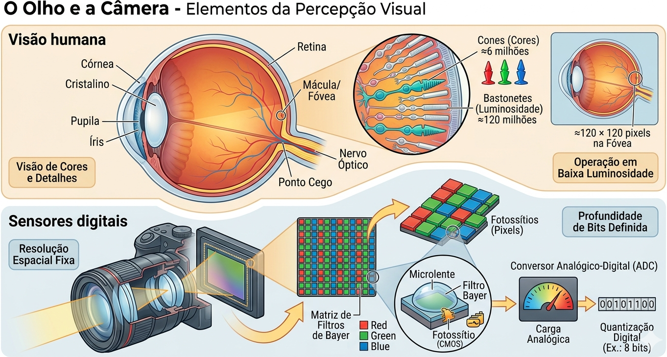
The formation of a digital image begins with the capture of light reflected by objects. As illustrated in Figure 2.1, both the human eye and digital cameras follow similar optical principles to focus light onto a sensitive surface, although they employ distinct biological and electronic mechanisms for signal transduction.
2.2.1 Human vision
The eye functions as a complex optical system: light passes through the cornea, the aqueous humor, the pupil (controlled by the iris), and the lens — which adjusts focus dynamically — until it reaches the retina. In the retina, photoreceptors are found: the cones (≈6 million), concentrated in the fovea, are responsible for color and detail vision, while the rods (≈120 million) ensure vision under low illumination (scotopic vision), detecting only shades of gray. The blind spot is the region from which the optic nerve originates, lacking receptors.
2.2.2 Digital sensors
In cameras, image sensors play the role of the retina. The two most common types are the CCD (Charge-Coupled Device) and the CMOS (Complementary Metal-Oxide-Semiconductor). The sensor is composed of an array of photosites (pixels) that accumulate electrical charge proportional to the incident light.
For color reconstruction, the Bayer Filter is used, a matrix of color filters that allows each pixel to capture only one color component: red, green, or blue (RGGB - Red, Green, Green, Blue). Subsequently, an ADC (Analog-to-Digital Converter) quantizes this charge into numerical values, defined by a bit depth (e.g., 8 bits, resulting in 256 intensity levels).
NoteCuriosity
Although the human eye has millions of receptors, high-definition resolution is confined to the fovea (central vision), equivalent to approximately \(120 \times 120\) pixels. The perception of a complete scene in high resolution is the result of intensive post-processing performed by the brain.
Figure 2.1: Didactic comparison between the biological and electronic visual systems: at the top, the anatomy of the human eye highlighting the retina and photoreceptors (cones and rods); below, the structure of a digital camera detailing the CMOS sensor, the Bayer filter array (RGGB), and the digital quantization process carried out by the ADC.
2.3 Optical Illusions: The Challenges of Visual Perception
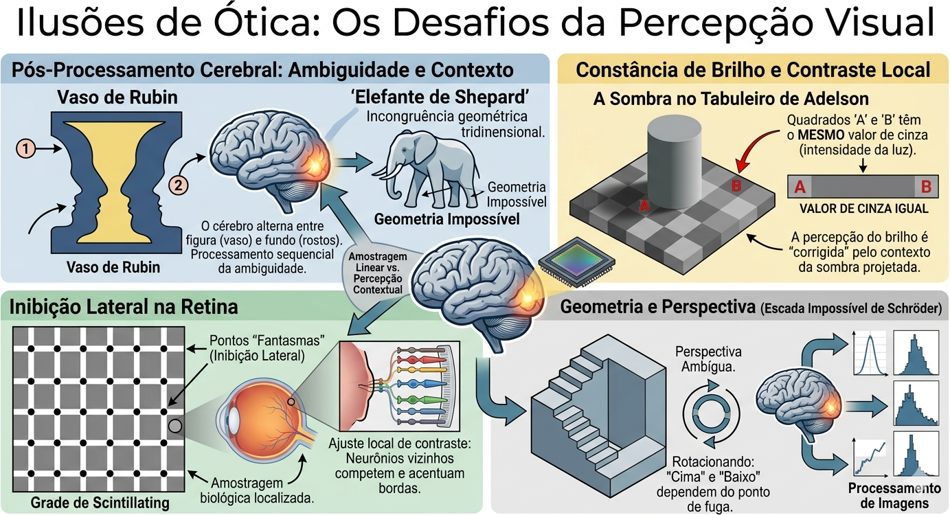
While digital sensors capture light intensity in a linear and objective manner, the human visual system interprets the scene based on context, prior experiences, and biological survival mechanisms. Optical illusions are not “errors” of the eye but evidence of the intense brain post-processing carried out in the visual cortex.
2.3.1 Ambiguity and Context
The brain constantly seeks to make sense of ambiguous patterns. In the example of the Rubin Vase (see Figure 2.2), perception alternates between the figure (vase) and the background (two faces), demonstrating that we cannot process both interpretations simultaneously. The Shepard Elephant illusion, in turn, plays on our inability to reconcile contour lines that suggest volume in logically impossible positions.
2.3.2 Brightness and Local Contrast
Many illusions arise from lateral inhibition, a mechanism by which neighboring neurons in the retina compete with one another to enhance edges. In the Scintillating Grid, “ghostly” dark spots seem to appear at the white intersections due to this local contrast processing.
The Adelson Checker Shadow illusion is perhaps the most striking for computer vision: square “A” and square “B” have exactly the same gray value in the sensor (or digital file), but the brain “corrects” the brightness of “B” by understanding that it lies under a cast shadow, perceiving it as lighter.
2.3.3 Geometry and Perspective
Depth perception can be deceived by geometric constructions that challenge three-dimensional logic from a specific viewing angle. The Schröder Staircase exploits perspective ambiguity to create an object that appears to ascend or descend depending on how it is observed, highlighting how our interpretation of “up” and “down” depends on the vanishing point.
An image can be modeled as the product of two functions:
\[
f(x,y) = i(x,y) \cdot r(x,y)
\tag{2.1}\]
where:
\(i(x,y)\) is the illumination incident upon the scene (light energy per unit area), determined by the light source;
\(r(x,y)\) is the reflectance of the object (fraction of reflected light), determined by the optical properties of the surface, with \(0 < r(x,y) < 1\).
In practice, the two components vary at distinct spatial scales: \(i(x,y)\) tends to vary slowly across space, whereas \(r(x,y)\) may exhibit abrupt variations associated with textures, edges, and fine details. Digital image processing (DIP) techniques often seek to separate or compensate for these components, as in methods for non-uniform illumination correction.
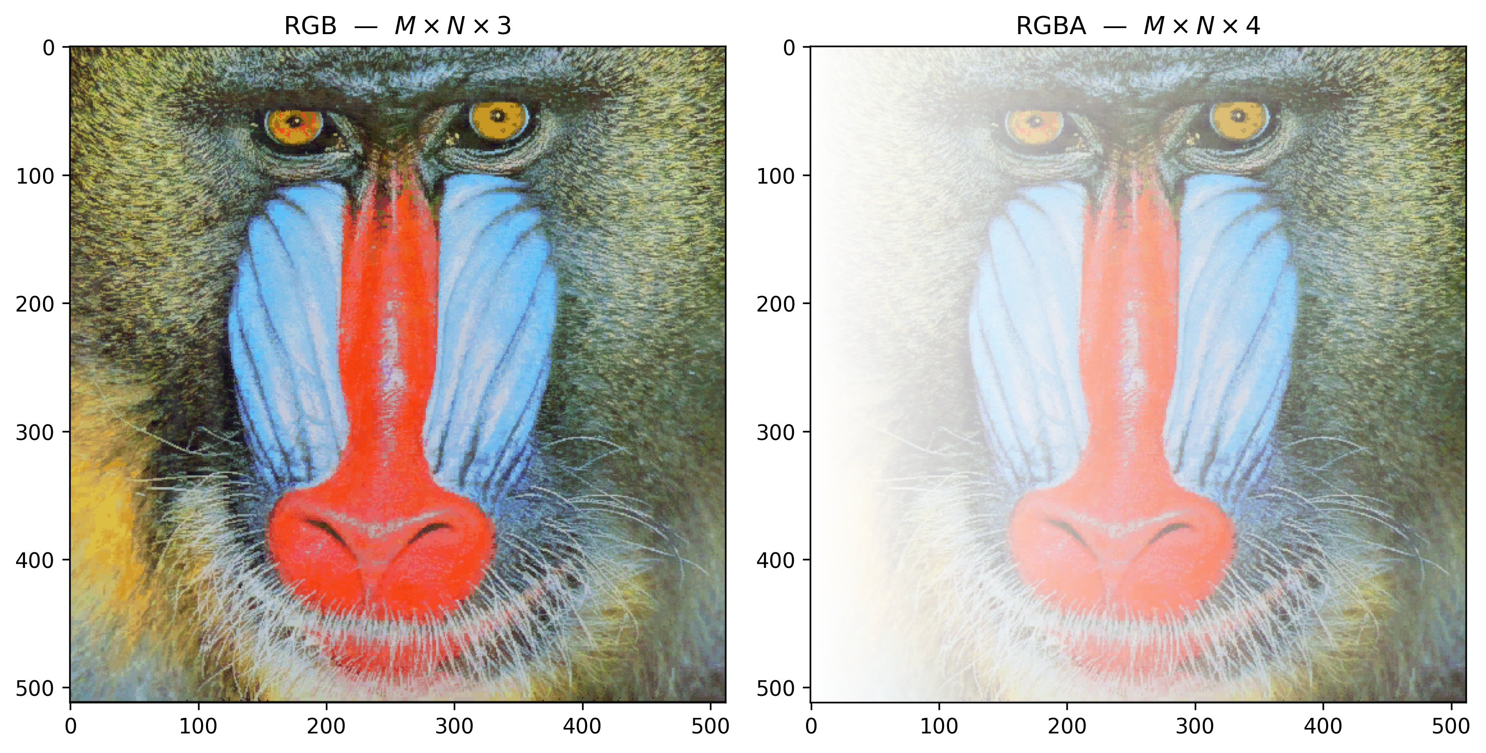
Figure 2.3 illustrates how this model manifests in digital color images, represented by multiple spectral channels (RGB) and, optionally, by an additional transparency channel (RGBA).
2.4.1 Digital Representation and Spectral Channels
In digital color images, the function \(f(x,y)\) from Equation 2.1 is represented by multiple spectral channels. In the RGB standard, each pixel stores three independent samples:
where \(A(x,y)\) represents the alpha channel, responsible for encoding the pixel’s opacity. By convention, the value \(A = 0\) indicates a fully transparent pixel, while \(A = 255\) (or \(1\)) represents a fully opaque pixel.
Thus, a digital color image is structured as a multidimensional matrix with dimensions:
RGB:\(M \times N \times 3\)
RGBA:\(M \times N \times 4\)
where each position \((x,y)\) stores the samples associated with the optical properties of that spatial coordinate.
The conversion between intensity ranges is straightforward and given by:
\[f_{\text{norm}}(x,y) = \frac{f(x,y)}{255}\]
where \(f(x,y) \in [0,\,255]\) and \(f_{\text{norm}}(x,y) \in [0,\,1]\).
Scale Convention Across Libraries: Different programming ecosystems adopt distinct value ranges and orderings to represent digital channels, as summarized in Table 2.1.
Table 2.1: Scale and channel order conventions in major DIP libraries.
Library
Default type
Value range
Band order
Array/tensor shape
OpenCV
uint8
\([0, 255]\)
BGR
\(H \times W \times C\)
Pillow
uint8
\([0, 255]\)
RGB
\(H \times W \times C\)
NumPy
uint8/float32
\([0,255]\) or \([0,1]\)
—
\(H \times W \times C\)
scikit-image
float64
\([0{,}0,\;1{,}0]\)
RGB
\(H \times W \times C\)
PyTorch
float32
\([0{,}0,\;1{,}0]\)
RGB
\(C \times H \times W\)
TensorFlow/Keras
float32
\([0{,}0,\;1{,}0]\)
RGB
\(H \times W \times C\)
Neglecting these discrepancies is a frequent source of errors in CV workflows — such as, for example, feeding an image read via OpenCV (BGR default, uint8 type) directly into a deep PyTorch model that assumes the normalized RGB format.
2.4.2 Preparing the Practical Environment
The following block loads the morph.py module from the repository and demonstrates, for a synthetic pixel, the different scaling conventions and channel orders adopted by the main image processing libraries.
The following excerpt displays the source code of the mm.read function, allowing you to directly verify how the morph.py library implements image reading.
import inspectprint(inspect.getsource(mm.read))
    @staticmethod
    def read(file, pil=False, grayscale=False):
        """Lê imagem (local, URL ou Google Drive) → PIL.Image, ndarray 2D ou RGB 3D."""
        import re, requests
        from PIL import Image
        from io import BytesIO
        from urllib.request import urlopen, Request
        np = mm._get_np()

        # — fonte: URL / Google Drive —
        if isinstance(file, str) and file.startswith(("http://", "https://", "id=")):
            m = re.search(r"id=([\w-]+)", file) or re.search(r"/d/([\w-]+)", file)
            url = f"https://drive.google.com/uc?export=view&id={m.group(1)}" \
                if m and ("id=" in file or "drive.google.com" in file) else file
            hdr = {"User-Agent": "Mozilla/5.0 AppleWebKit/537.36 Chrome/124 Safari/537.36"}
            try:
                r = requests.get(url, headers=hdr, timeout=20)
                if r.status_code == 429: raise requests.exceptions.HTTPError()
                r.raise_for_status()
                file = BytesIO(r.content)
            except:
                file = BytesIO(urlopen(Request(url, headers=hdr), timeout=20).read())

        img = Image.open(file)
        img.load()
        if pil:                    return img
        if grayscale:              return np.array(img.convert("L"))   # (H,W)
        if img.mode == "L":        return np.array(img)                # (H,W)
        if img.mode == "RGBA":                                         # fundo branco
            bg = Image.new("RGB", img.size, (255, 255, 255))
            bg.paste(img, mask=img.split()[3])
            return np.array(bg)
        return np.array(img.convert("RGB"))                            # (H,W,3)
2.4.4 RGB and RGBA: Practical Example with the Mandrill Image
The following example loads the Mandrill image in RGB format, artificially constructs an alpha channel with a horizontal gradient, and displays both representations, concretely illustrating the matrix structures \(M \times N \times 3\) and \(M \times N \times 4\).
Figure 2.3: RGB image (3 channels, \(M \times N \times 3\)) and RGBA version (4 channels, \(M \times N \times 4\)) with gradual alpha transparency from left to right. Mandrill image — USC SIPI Image Database (public domain).
2.5 Digitization: Sampling and Quantization
To transform a continuous scene into a digital image, two processes are required: sampling and quantization.
2.5.1 Sampling - Discretization of Space
Sampling consists of measuring the value of the function \(f(x,y)\) at equally spaced points, forming a matrix of \(M\) rows (height) and \(N\) columns (width). Each element of this matrix is a pixel. The spatial resolution is given by \(M \times N\). The higher the resolution, the more spatial details are preserved, but also the greater the computational and storage cost.
2.5.2 Quantization - Discretization of Intensity
Quantization assigns to each pixel a discrete numerical value, usually represented by an integer of \(b\) bits. The bit depth defines the number of intensity levels: \(2^b\). Grayscale images typically use 8 bits (256 levels). Color images use three 8-bit channels (24 bits in total).
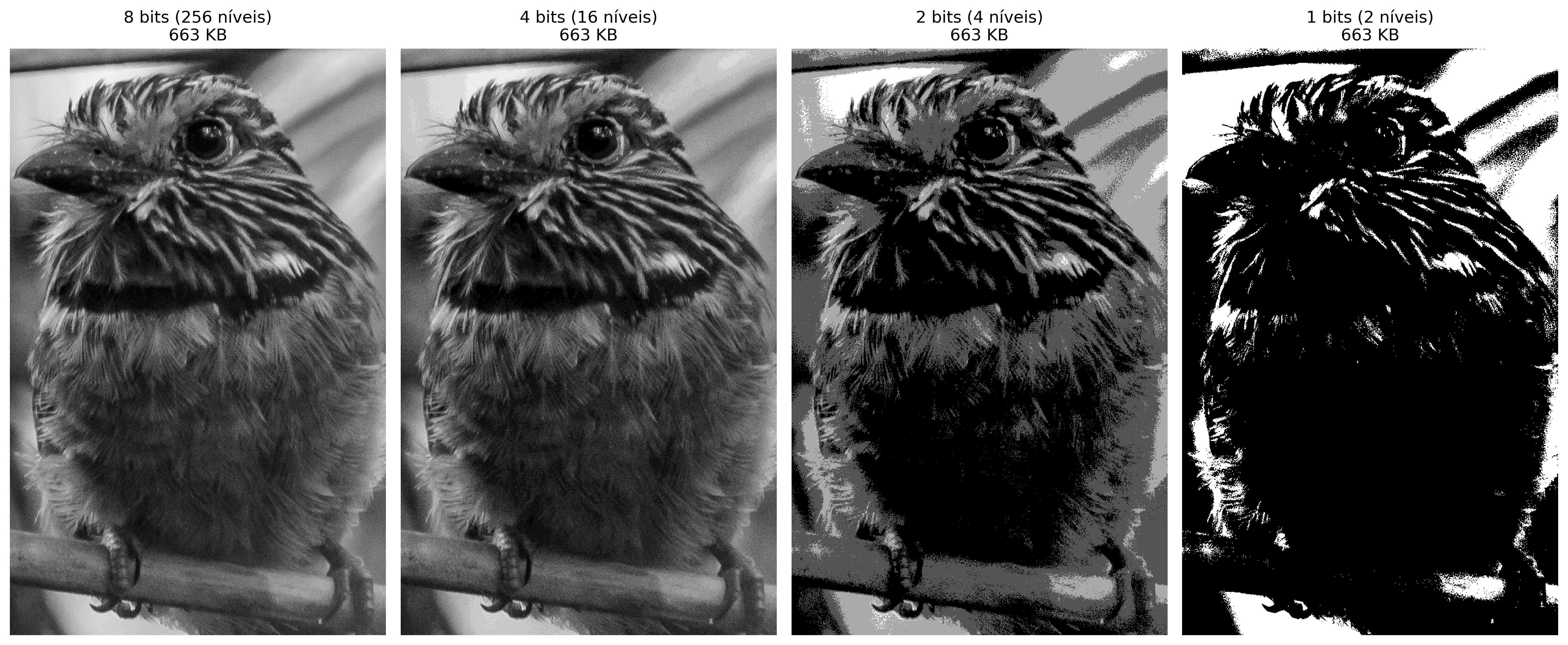
Illustration: If we use only 1 bit per pixel (black and white), we lose all intermediate tones. With 2 bits (4 levels), coarse gradients are already noticeable. With 8 bits, the human eye can hardly perceive the discretization (continuous vision).
WarningQuantization Error
Quantization error is the difference between the actual analog value and the assigned discrete value. It manifests as quantization noise, visible in regions with smooth gradients when few bits are used.
2.5.3 Effects of Sampling and Quantization
The following experiments show how reducing spatial resolution (subsampling) and bit depth degrade visual quality. Use the code to explore different factors and gray levels.
# Example image (striped-bearded) — basis for the sampling figures,# quantization and geometric transformations of this chapter.base ="https://upload.wikimedia.org/wikipedia/commons"arquivo = ("Area_de_Prote%C3%A7%C3%A3o_Ambiental_""Quilombos_do_M%C3%A9dio_Ribeira_-_Thomas-""Fuhrmann_%282023-_02%29_Malacoptila_striata.jpg")url =f"{base}/c/c5/{arquivo}"caminho ="imagens/barbudo-rajado.jpg"ifnot os.path.exists(caminho): os.makedirs("imagens", exist_ok=True) mm.write(mm.read(url), caminho)img_color = mm.read(caminho)img_gray0 = mm.gray(img_color)img_gray = mm.crop(img_gray0, 820, 1850, 890, 1550) # crop to see detailsprint(f"Original image: {img_color.shape}")
Original image: (3067, 2047, 3)
import numpy as np# Reinterpretation as a PIL object to access EXIF metadata (Python only).img_pil = mm.read(caminho, pil=True) # returns PIL Image with EXIFimg_numpy = np.array(img_pil)exif = img_pil._getexif() # now it works — img_pil is PIL Imageprint(f"Image type: {type(img_color)}")
Image type: <class 'numpy.ndarray'>
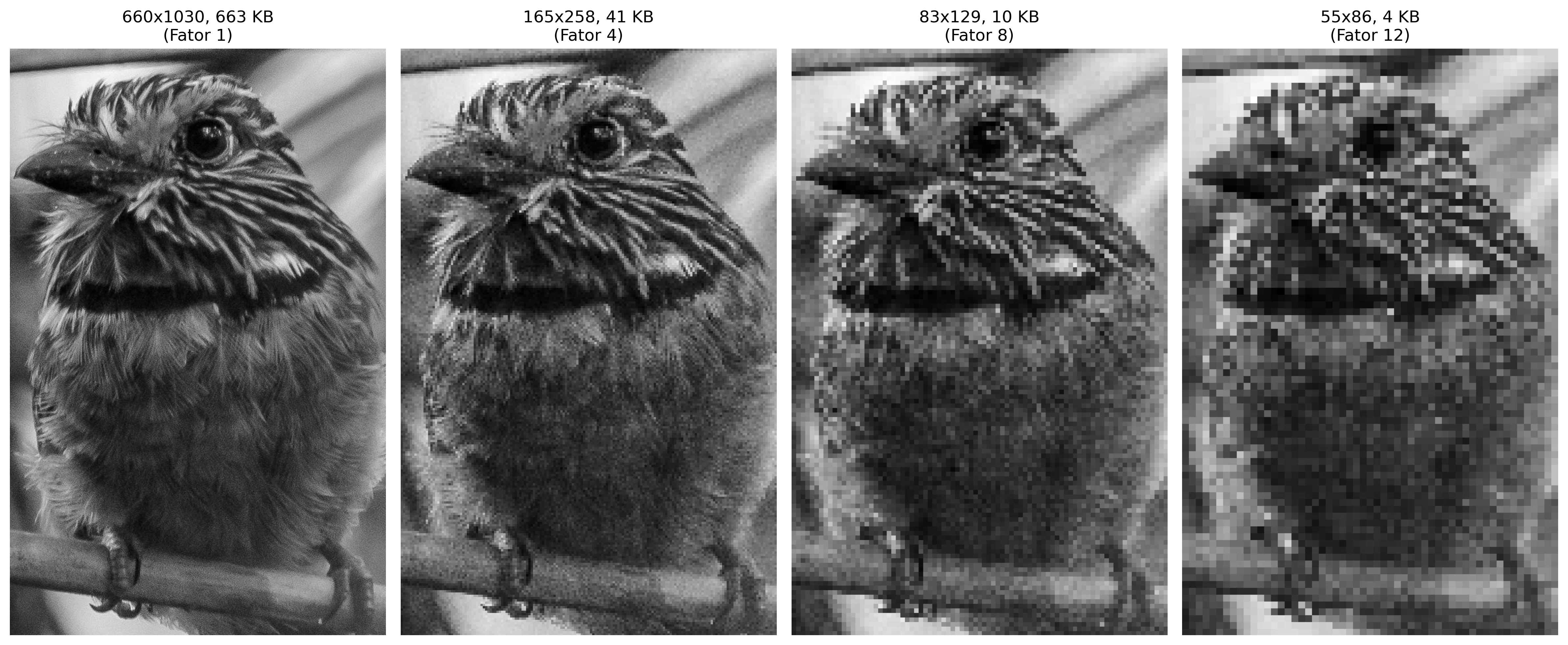
The experiment presented in Figure 2.4 illustrates the trade-off between spatial resolution and storage cost in memory. The code employs the subsampling technique via slicing to reduce the original pixel matrix according to a factor \(f\), resulting in memory savings — for example, a factor \(f=8\) reduces the data size by 64 times (\(8^2\)). For visual comparison purposes, the reduced images are restored to their original dimensions (\(512 \times 512\)) through nearest-neighbor interpolation (nearest). This process does not recover the lost information, but it makes evident the effect of aliasing and the block structure (pixelation) generated by the low data density of the sampled matrix.
def subsample_simple(image, f):# Subsampling via slicing reduced = mm.subsample(image, f)# Memory calculation in KB mem_kb = reduced.nbytes /1024 label =f"{reduced.shape[1]}x{reduced.shape[0]}, {int(mem_kb)} KB\n(Fator {f})"# Restores the size for display (original H, W) res = mm.resize(reduced, (image.shape[1], image.shape[0]), method='nearest')return res, labelfactors = [1, 4, 8, 12]# Generates the results and splits them into lists for mm.showresults = [subsample_simple(img_gray, f) for f in factors]imgs_list = [r[0] for r in results]titles_list = [r[1] for r in results]mm.show(imgs_list, titles=titles_list, cols=4, figsize=(16, 12))
Figure 2.4: Effect of subsampling. The titles display the dimensions (W x H) and the size of the array in memory (KB).
The experiment in Figure 2.5 focuses on intensity quantization, the process of discretizing the amplitude of the function \(f(x,y)\). While subsampling affects the spatial grid, reducing the bit depth limits the number of gray levels available to represent brightness.
By reducing the depth from 8 bits (256 levels) to smaller values, the posterization effect arises, where smooth gradients in a scene are replaced by abrupt transitions. At the 1-bit limit, the image becomes strictly binary, preserving only the silhouette and losing texture and volume details.
def quantize_simple(image, bits):"""Reduces bit depth and computes memory metadata.""" levels =2** bits# Normalization and uniform quantization quantized = (np.floor(image /256* levels) / levels *255).astype(np.uint8)# Memory calculation in KB mem_kb = quantized.nbytes /1024 label =f"{bits} bits ({levels} níveis)\n{int(mem_kb)} KB"return quantized, label# List of bits to test (8 is the default, 1 is binary)bits_test = [8, 4, 2, 1]# Generates results and separates into lists for mm.showresults_q = [quantize_simple(img_gray, b) for b in bits_test]imgs_q = [r[0] for r in results_q]titles_q = [r[1] for r in results_q]mm.show(imgs_q, titles=titles_q, cols=4, figsize=(16, 12))
Figure 2.5: Effect of reducing bit depth. The titles display the number of bits, levels, and size in memory (KB).
2.5.4 Technical Analysis
Domain vs. Codomain: Note that the spatial resolution (matrix dimensions) remains constant at 512x512; only the codomain of the image function changes.
Memory Constancy: Observe in the titles that the size in KB does not decrease. This occurs because NumPy stores each quantized pixel in an 8-bit container (uint8), regardless of whether the actual value is only 0 or 1.
Perception: Visual degradation becomes critical below 4 bits, where the human eye begins to perceive the artificial “boundaries” created by the lack of intermediate tones.
The limitation of data types smaller than a byte in the Python/NumPy ecosystem stems from hardware architecture, which addresses memory in blocks of 8 bits (Bytes). To maintain compatibility with OpenCV and ensure efficiency, even binary elements are mapped to 1-byte containers (uint8 or bool8).
Although languages such as ANSI C allow the packing of 8 pixels per byte (bit-packing), this approach requires constant unpacking for computations and imposes high complexity in pointer manipulation. As per Table 2.2, the use of uint8 is favored for ease of neighbor access and versatility in geometric transformations. Furthermore, native NumPy and OpenCV methods execute processing internally at a low level (C/C++), making vectorized operations faster than manual implementations with nested loops in Python.
Table 2.2: Comparison between packing strategies and processing efficiency.
Feature
Python (NumPy/OpenCV)
ANSI C (Bit-packing)
Smallest Unit
1 Byte (8 bits)
1 Bit
Memory (Binary)
256 KB (for 512x512)
32 KB (for 512x512)
Speed
High (C vectorization)
Variable (Slow if bit-shifting)
Complexity
Low: Ready-made methods
High: Pointers and Masks
2.6 Relationships Between Pixels - Image Topology
Pixels are not isolated elements; their relative positions define important concepts for processing.
2.6.1 Neighborhood
Given a pixel with coordinates \((x,y)\), two main types of neighborhood are defined (for images on a rectangular \(grid\)):
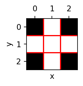
4-Neighborhood (von Neumann): includes the pixels at positions \((x-1,y)\), \((x+1,y)\), \((x,y-1)\), \((x,y+1)\).
8-Neighborhood (Moore): includes all eight adjacent pixels (adds the four diagonal ones).
The choice of neighborhood influences operations such as edge detection, gradient computation, and connectivity.
# # Creation of a 3x3 matrix for topological example# viz = np.zeros((3, 3), dtype='uint8')# # Defining Neighborhood-4 (N4) with a different value for emphasis# viz[0, 1] = viz[2, 1] = viz[1, 0] = viz[1, 2] = viz[1, 1] = 255# or simply (test with numbers as arguments):viz = mm.secross()# Display of the matrix for coordinate analysismm.drawImgPlt(viz, scale=40)
Figure 2.6: Illustration of 4-neighborhoods in a 3x3 matrix. At the center (1,1), the pixel of interest.
import importlibimport morphimportlib.reload(morph)from morph import mm
2.6.2 Adjacency, connectivity, and paths
Two pixels are adjacent if they are in contact according to a defined neighborhood and satisfy a value criterion (e.g., same intensity level). A connectivity defines an equivalence relation between pixels that form a connected region. A path is a sequence of adjacent pixels.
4-connectivity (N4) and 8-connectivity (N8) can produce different results in segmentation and in the computation of connected components (labeling). For example, a checkerboard pattern can be completely disconnected under N4 but fully connected under N8.
2.6.3 Distances Between Pixels
Distance metrics are fundamental for quantifying physical proximity and connectivity among the elements that make up the digital grid. As demonstrated in Table 2.3, the choice of metric defines the movement cost between pixels and alters the behavior of segmentation algorithms and morphological analysis.
To measure the distance between two pixels \(p(x_1, y_1)\) and \(q(x_2, y_2)\), different metric functions are used, each imposing distinct movement constraints on the grid:
Table 2.3: Comparison of distance metrics applied to the pixel grid.
Metric
Definition
Interpretation
Euclidean
\(\sqrt{(x_1-x_2)^2 + (y_1-y_2)^2}\)
Exact straight-line distance (continuous)
Manhattan (City block)
\(|x_1-x_2| + |y_1-y_2|\)
Horizontal + vertical movements
Chebyshev (Chessboard)
\(\max(|x_1-x_2|, |y_1-y_2|)\)
Largest displacement among the axes
These distances are applied in various DIP contexts, including geometric interpolation algorithms, distance transforms, region growing, and shape analysis.
NotePractical Example
Considering two pixels with relative displacements \(\Delta x = 3\) and \(\Delta y = 4\):
Euclidean: \(\sqrt{3^2 + 4^2} = 5\) (hypotenuse of the right triangle).
Manhattan: \(3 + 4 = 7\) (sum of the legs).
Chebyshev: \(\max(3, 4) = 4\) (dominance of the largest displacement).
2.7 Image Storage
The choice of file format is a decisive step in the processing pipeline, as it determines how sampling and quantization data will be preserved or discarded. As presented in Table 2.4, each extension balances data fidelity and storage efficiency in a distinct manner.
Table 2.4: Main digital image storage formats and their applications in DIP.
Format
Characteristics
Typical Use
PGM
Simple grayscale map format (text or binary).
Academic research and Unix tools.
BMP
Uncompressed (or simple compression).
Windows, legacy applications.
PNG
Lossless compression.
Web, images with transparency.
JPEG
Lossy compression, ideal for photographs.
Photos, digital cameras.
TIFF
Supports multiple layers and varied compression.
Publishing, archiving.
RAW
Raw sensor data, unprocessed.
Professional photography.
DICOM
Medical standard with embedded clinical metadata (patient, equipment, protocol).
Radiology, tomography, magnetic resonance imaging.
Image metadata includes parameters such as width, height, bit depth, and color encoding. In scientific formats, calibration information and capture details are also preserved. When using the mm.read() function, the morph library automatically preserves this data so that the original properties of the image are respected.
In scientific and hospital contexts, the DICOM (Digital Imaging and Communications in Medicine) standard is favored to ensure that there is no loss of diagnostic precision. Public repositories such as The Cancer Imaging Archive (TCIA), the Alzheimer’s Disease Neuroimaging Initiative (ADNI), and PhysioNet provide vast datasets in this format, including anonymized clinical metadata that is essential for scientific research.
2.7.1 Example: Metadata Extraction and GPS Location
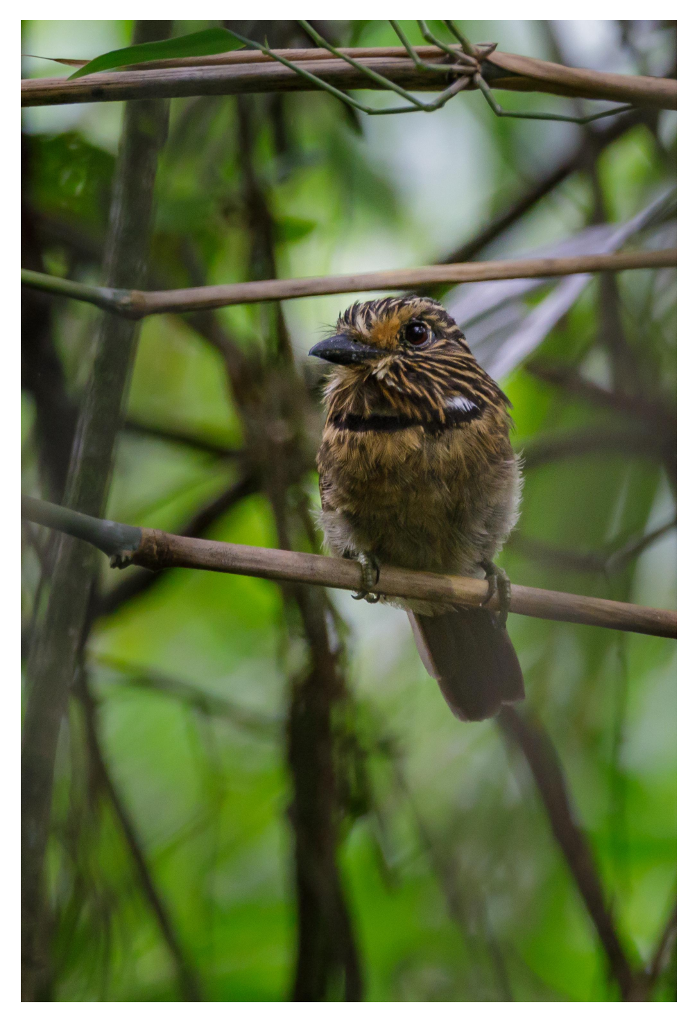
Unlike the pure pixel matrix obtained through conventional reading—as in the bird image presented at the beginning of this chapter—the use of the pil=True argument in the mm.read() method changes the nature of the returned object (see Figure 2.7). While the default (pil=False) returns an RGB numpy.ndarray, reading with pil=True returns a specialized object from the Pillow library, capable of interpreting the EXIF header.
The EXIF header (Exchangeable Image File Format) functions as a technical repository of the capture, allowing the Pillow object to interpret a vast range of information that goes far beyond GPS coordinates. By using pil=True, the system gains access to the “DNA” of the image, including hardware metadata (camera brand and model), optical settings (aperture, focal length, and exposure time), and lighting parameters (flash usage and white balance).
This distinction is important in digital image processing, as it transforms the sampling matrix into a contextualized dataset, where the physical characteristics of the sensor and lens can be used to normalize brightness or correct geometric distortions.
from PIL.ExifTags import TAGSimport os, numpy as npbase ="https://upload.wikimedia.org/wikipedia/commons"arquivo = ("Area_de_Prote%C3%A7%C3%A3o_Ambiental_""Quilombos_do_M%C3%A9dio_Ribeira_-_Thomas-""Fuhrmann_%282023-_02%29_Malacoptila_striata.jpg")url =f"{base}/c/c5/{arquivo}"caminho ="imagens/barbudo-rajado.jpg"# 1. Reading — preserves PIL object with EXIFifnot os.path.exists(caminho): os.makedirs("imagens", exist_ok=True) img_obj = mm.read(url, pil=True) mm.write(img_obj, caminho) # saving preserving EXIFelse: img_obj = mm.read(caminho, pil=True)img_numpy = np.array(img_obj) # conversion to NumPy# 2. GPS extraction and conversion (Tag 34853)exif = img_obj._getexif()if exif and (gps := exif.get(34853)): to_dec =lambda dms, ref: float(-(dms[0]+dms[1]/60+dms[2]/3600) if ref in'SW'else (dms[0]+dms[1]/60+dms[2]/3600)) lat, lon = to_dec(gps[2], gps[1]), to_dec(gps[4], gps[3])print(f"GPS Decimal: {lat:.6f}, {lon:.6f}")print(f"Maps: https://www.google.com/maps/search/?api=1&query={lat},{lon}")# 3. Diagnosis of types, dimensions and pixel accessprint(f"\nPIL Type : {type(img_obj)} | Dimensions (x,y): {img_obj.size}")print(f"Pillow (0,0): {img_obj.getpixel((0, 0))}")print(f"NumPy Type: {type(img_numpy)} | Dimensions [y,x,c]: {img_numpy.shape}")print(f"NumPy [0,0]: {img_numpy[0, 0]}")# 4. Displaymm.show(img_numpy, scale=30)
Figure 2.7: Environmental Protection Area Quilombos of Médio Ribeira - Barbudo-rajado (Malacoptila striata). Credit: Thomas Fuhrmann (CC BY-SA 4.0).
NotePedagogical Note: The Subtle Difference in Dimensions
Notice that the representation of dimensions changes depending on the data structure used:
In Pillow (.size): Returns (Width, Height) — in the example: (2047, 3067). This is a view oriented toward the image file.
In NumPy (.shape): Follows the mathematical matrix convention: (Rows/Height, Columns/Width, Channels) — in the example: (3067, 2047, 3).
This distinction is fundamental to avoid indexing errors when implementing manual filters. While the Pillow object carries the “where” and “when” (context), the NumPy array carries the “how much” light (intensity) at each point of the image.
2.7.2 Why Is This Separation Important?
When loading an image through the conventional path (pil=False), the result is a numpy.ndarray, which strictly contains the numerical values resulting from quantization and sampling. However, when using pil=True, the mm.read() returns an object of class PIL.JpegImagePlugin.JpegImageFile.
This class keeps the file “open” to allow access to the capture context before the data are converted into a raw matrix. Note that the pixel at (0, 0) is identical in both representations — (58, 96, 0) in Pillow and [58, 96, 0] in NumPy — confirming that both describe the same data, only with different interfaces. This separation is vital: pixels serve algorithms; metadata serve georeferencing, scientific cataloging, and corrections based on the acquisition hardware.
To inspect all EXIF metadata of a Pillow object:
from PIL import ExifTagsexif_raw = img_obj._getexif()if exif_raw:for tag_id, valor insorted(exif_raw.items()): tag_nome = ExifTags.TAGS.get(tag_id, f"TAG_{tag_id}")print(f" {tag_nome:40s} : {valor}")
2.8 Basic Geometric Transformations
Geometric transformations alter the position of pixels while maintaining intensity values. They are fundamental for alignment, distortion correction, and data augmentation in machine learning.
An affine transformation is any mapping that preserves collinearity (points on a line remain on a line) and ratios of distances between collinear points. In 2D, every affine transformation can be expressed in homogeneous coordinates by a \(3 \times 3\) matrix:
The upper-left \(2 \times 2\) submatrix \(\mathbf{A} = \begin{bmatrix} a_{11} & a_{12} \\ a_{21} & a_{22} \end{bmatrix}\) controls rotation, scaling, and shearing; the vector \((t_x, t_y)^\top\) controls translation. The most commonly used geometric transformations in DIP — translation, rotation, and scaling — are special cases of \(\mathbf{T}\), and can be composed through matrix multiplication, in the order \(\mathbf{T} = \mathbf{T}_n \cdots \mathbf{T}_2 \mathbf{T}_1\).
NoteInverse transformation and interpolation
In practical implementation (cv2.warpAffine), the inverse transformation is applied: for each pixel \((x', y')\) of the destination image, the source position \((x, y) = \mathbf{T}^{-1}(x', y')\) is computed and the value is interpolated. This avoids holes in the resulting image caused by directly mapping integer pixels to non-integer positions.
2.8.1 Translation
Translation is the simplest affine transformation: it shifts all pixels by a vector \((t_x, t_y)\). In homogeneous coordinates, it is expressed by the matrix:
The third row of the matrix ensures that the operation remains in affine space, allowing translation, rotation, and scaling to be combined by simple matrix multiplication. In practice, cv2.warpAffine uses only the first two rows (a \(2 \times 3\) matrix), since the third row is always \([0, 0, 1]\).
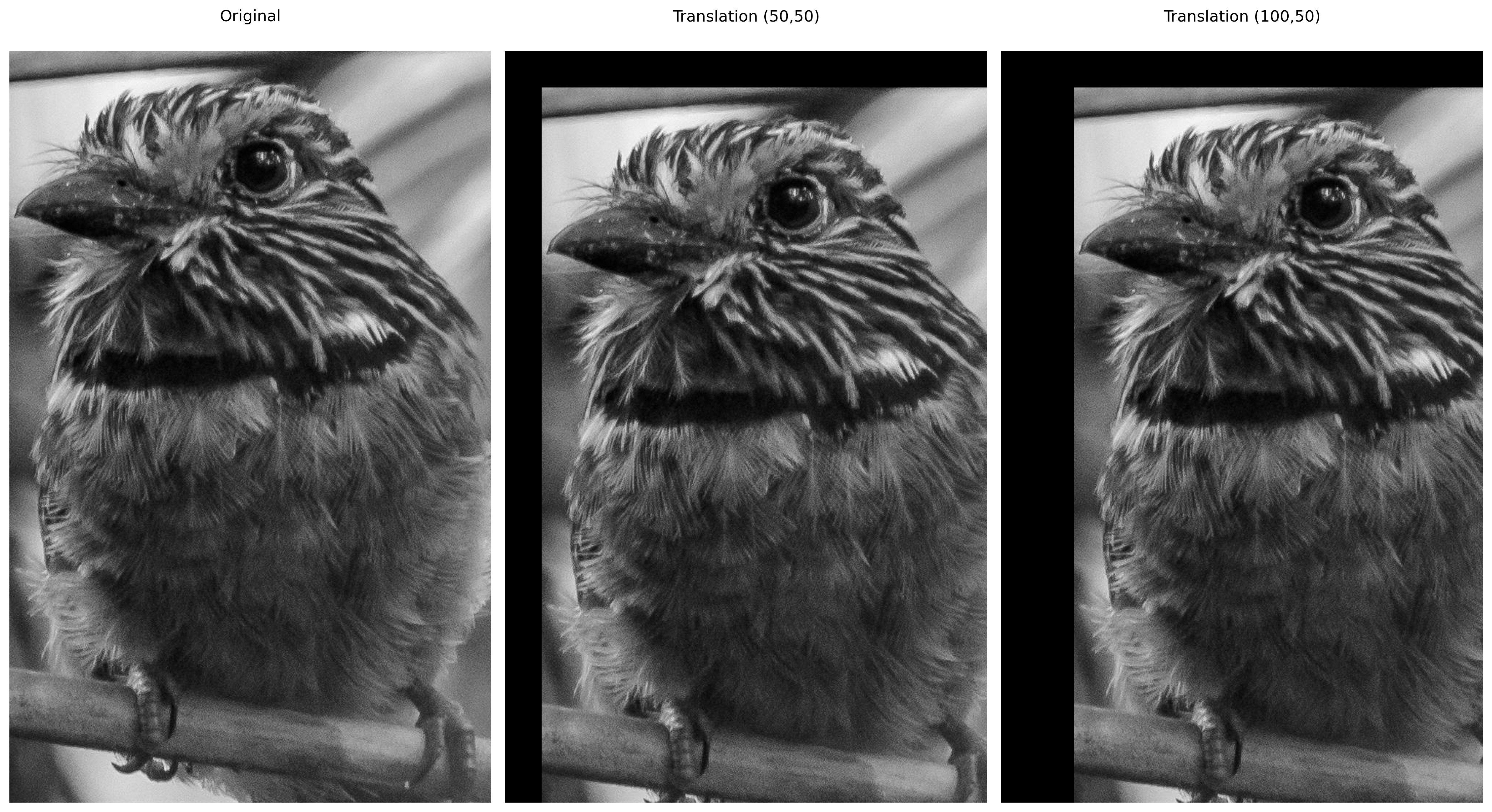
Pixels shifted beyond the original area are discarded; uncovered areas are filled with 0 (black). See an example in Figure 2.8.
Figure 2.8: Example of translation of the bird image with offsets (50,50) and (100,50).
2.8.2 Rotation
Rotation by angle \(\theta\) around a central point \((c_x, c_y)\) is composed of three affine transformations: translation to the origin, pure rotation, and translation back. The resulting matrix is:
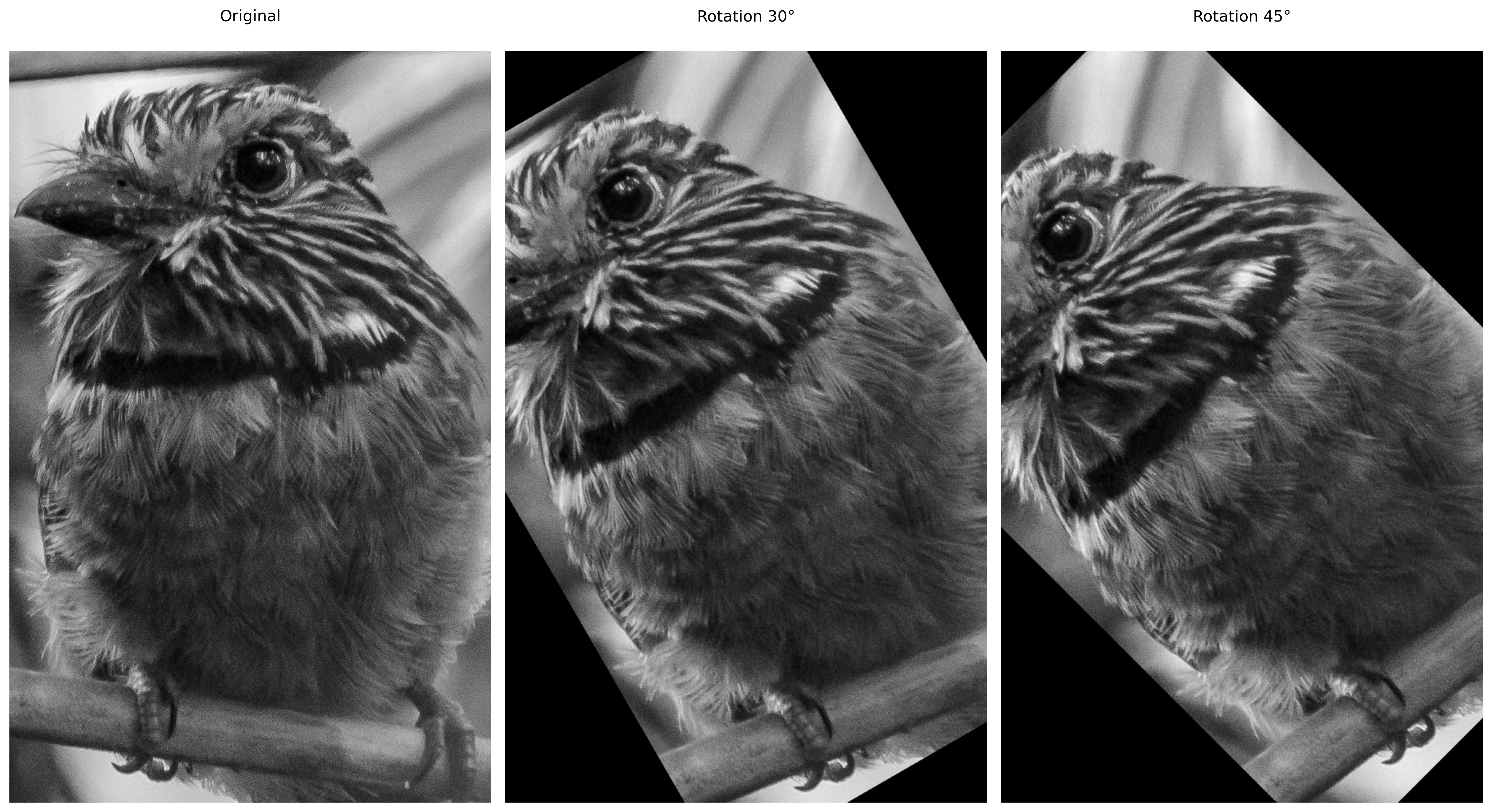
In the implementation, cv2.getRotationMatrix2D directly generates the first two rows of \(\mathbf{T}_{\text{rot}}\) (a \(2 \times 3\) matrix for warpAffine), also accepting a scale factor \(s\) that multiplies \(\cos\theta\) and \(\sin\theta\). See the example in Figure 2.9.
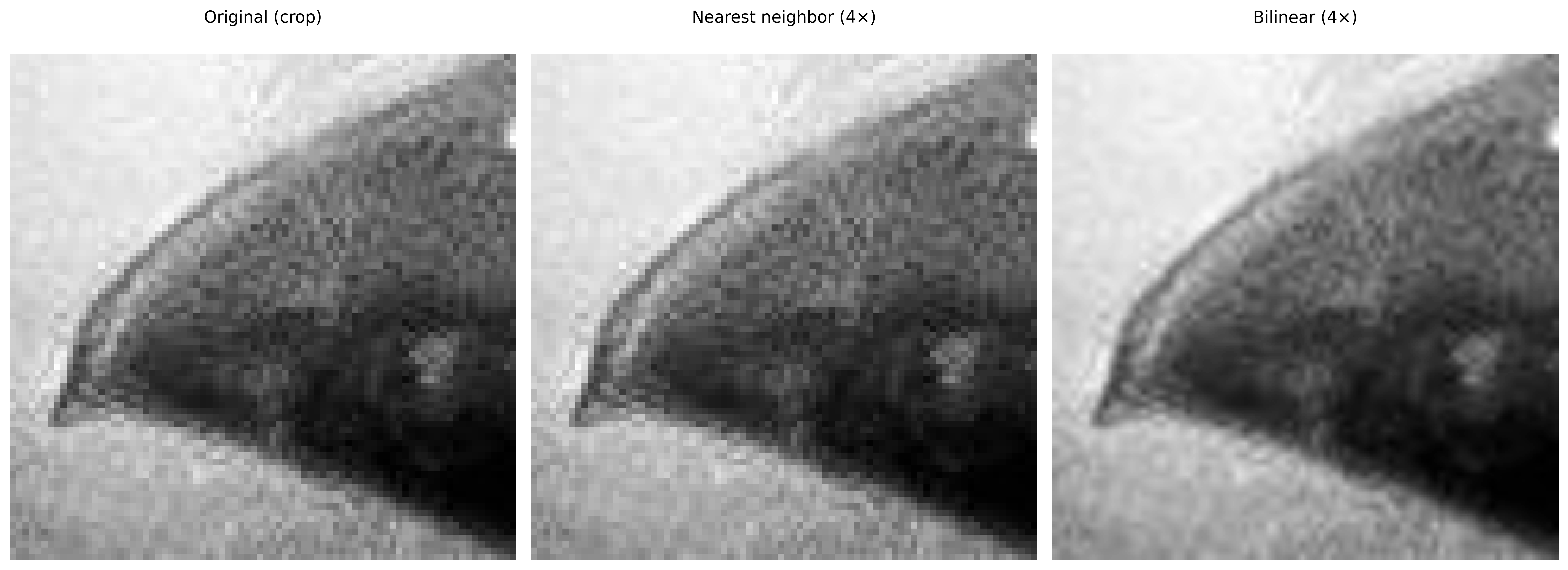
Since rotation moves pixels to new non-integer positions, cv2.warpAffine must estimate the color of each destination pixel from its neighbors — a process called interpolation. The interp parameter controls this behavior:
nearest (INTER_NEAREST): assigns the value of the nearest pixel. Fast, but produces jagged edges (aliasing) on diagonal borders.
bilinear (INTER_LINEAR, default): weighted average of the 4 nearest neighbors. Balances quality and performance — suitable for most cases.
bicubic (INTER_CUBIC): considers the 16 neighbors on a cubic surface. Produces smoother edges at the cost of greater processing.
When \(s > 1\) (enlargement), pixels of the destination image map to non-integer positions in the source — requiring interpolation to estimate the value. When \(s < 1\) (reduction), multiple source pixels contribute to a single destination pixel — requiring decimation. The same three methods described for rotation are available in mm.resize, with the difference that here the visual impact is more noticeable: in enlargement, nearest produces a blocky effect (pixelation), whereas bicubic better preserves edge sharpness, as shown in Table 2.5:
Table 2.5: Interpolation methods available in mm.resize and their respective numbers of neighbors used in the calculation.
Method
Neighbors used
Characteristic
'nearest'
1
Fast; produces a blocky effect (pixelation)
'bilinear'
4
Good quality/cost trade-off; smooth edges
'bicubic'
16
Greater sharpness; preferred in professional software
The size_or_factor parameter accepts either a scalar (uniform factor, e.g. 0.5 to reduce to half) or a tuple (width, height) for absolute dimensions.
Figure 2.10: Comparison of interpolation with zoom on the eye detail (60×60 crop, enlarged 4×). Note the blocky effect in nearest neighbor vs. the smoothing in bilinear.
2.8.4 Shearing
Shearing is an affine transformation that distorts the image by shifting each pixel proportionally to its position along one axis. The general matrix combines horizontal shear (\(sh_x\)) and vertical shear (\(sh_y\)):
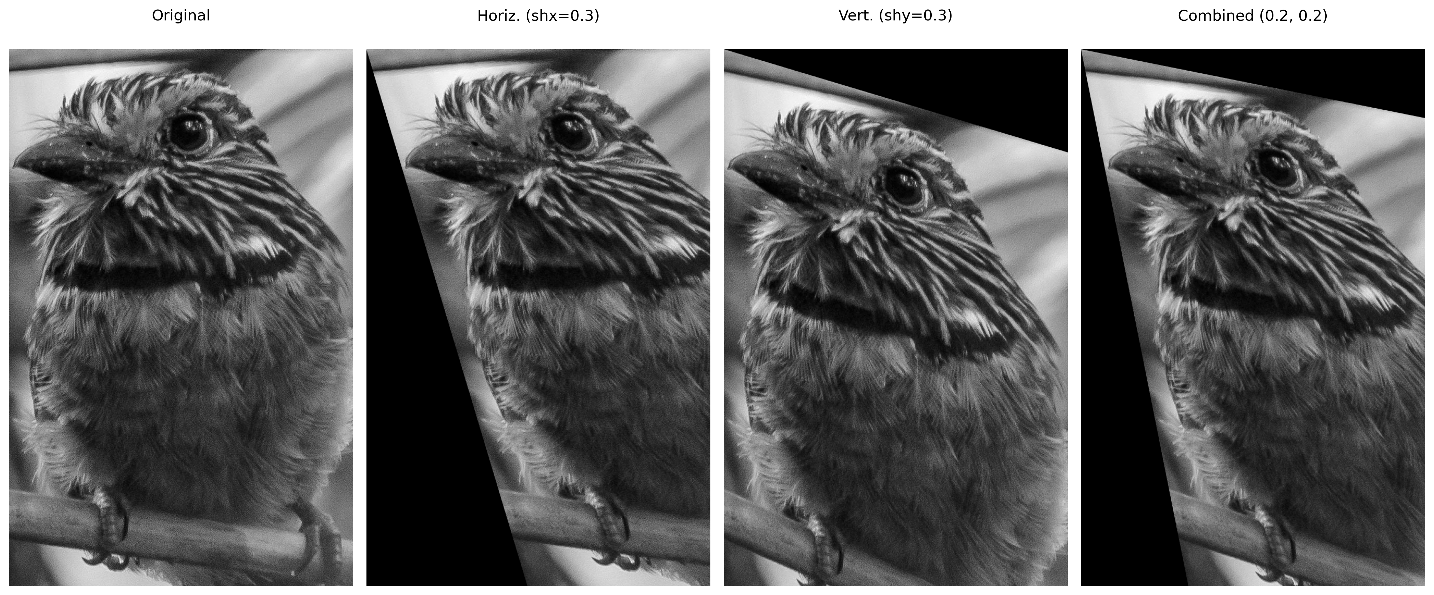
For \(sh_x \neq 0\) and \(sh_y = 0\), each row is shifted horizontally proportionally to its vertical position — producing the characteristic “tilt” effect. See the example in Figure 2.11.
Geometric transformations: translation, rotation, scaling (with bilinear or nearest-neighbor interpolation).
File formats: BMP, PNG, JPEG, TIFF, RAW; each with different trade-offs between quality and size.
Chapter 3 will address spatial operations such as convolution, filtering, and mathematical morphology (erosion, dilation).
2.10 🤖 Using Gemini Notebook as a Complementary Tutor
In this edition, we encourage the use of Gemini Notebook as a complementary learning tool. This AI tool relies exclusively on the documents provided by the author as its knowledge base, ensuring responses consistent with the book’s content.
For each chapter, we have prepared a specific project on the platform. For an enhanced study experience, use the access link below:
Important🎓 Study with the Intelligent Tutor
To interact with the content of this chapter, access the link below. The environment contains teaching materials in different formats, generated from the chapter’s PDF. On the platform, especially explore the Study Guide and Conversation options to deepen your understanding.
The project for this chapter in Gemini Notebook was built using only the text in Portuguese and code examples in Python. If you are studying from the English or French edition, or following the C++ track, the tutor’s responses may not exactly match the version you are reading.
⚠️ Notice on AI-Generated Content
AI is a powerful ally in studying, but the generated content may contain errors or inaccuracies. Always consult books, scientific articles, and other reliable academic sources to validate the information. Whenever possible, run the practical examples provided in this chapter to verify the results.
2.11 Exercise List
(15%) Explain, in your own words, the difference between sampling and quantization. Give a concrete example of each in the context of a digital image.
(15%) Consider an image with a spatial resolution of 1024 × 768 pixels and a bit depth of 24 bits (8 bits per RGB channel). Calculate the total uncompressed size of the image in bytes and in megabytes.
(20%) Using the laboratory code, modify the subsampling factor to 3 and to 6. Visually describe what happens to the edges of objects. What is the aliasing effect?
(20%) For the grayscale image, apply quantization with 3 bits (8 levels) and 5 bits (32 levels). Compare the results and explain why 5 bits can already be considered sufficient for many applications.
(15%) Given two pixels \(A=(10,20)\) and \(B=(15,25)\), calculate the Euclidean, Manhattan, and Chebyshev distances between them.
(15%) Using the mm.rotate function, rotate the bird image at angles of 90°, 180°, and 270° with bilinear interpolation. Compare this with rotation using method='nearest'. In which situations is nearest-neighbor interpolation still useful?
Chapter References
The theoretical foundation of this chapter is based on the following works:
Gonzalez (2018) for the concepts of sampling, quantization, and relationships between pixels.
Szeliski (2022) for geometric transformations and connectivity.
Bradski (2008) for the practical implementation with OpenCV and morph.py.
2.12 💻 Practical Part with Programming Exercises
🎯 Objective of this Notebook
The notebook allows you to develop, validate, organize, and test solutions for Programming Exercises (PEs) in interactive environments, such as Colab, with the same test cases as Moodle, copying them there only when it is time to record the official grade.
Download
Download morph.py and testsuite.py by running the cell below:
To evaluate the tests, run TestSuite("EP04_01.extension").run() in a new cell, replacing the extension with that of the language used (.py, .java, .c, .cpp, .js, or .r). The system downloads the test cases from GitHub, runs the program, and computes the grade automatically.
To test Python code directly, without saving a file, use run_code(code) by passing the code as a string in a variable code:
code ="""from morph import mm# ... your code here ..."""TestSuite("EP04_01").run_code(code)
2.12.1 EP02_01 ☀️ Brightness and Contrast Adjustment
In this activity, the goal is to implement a point operator for linear intensity transformation, applying dynamic brightness and contrast adjustment to a digital image.
2.12.1.1 📋 Implementation Guidelines
The algorithm should follow the execution flow below:
Dimensions: Read the integers \(L\) (rows) and \(C\) (columns) of the matrix.
Parameters: Read the real value \(\alpha\) (contrast factor) and the integer \(\beta\) (brightness factor).
Data: Read the integer values of the original matrix.
Mapping: For each pixel \(p\), compute the new value \(p'\) using the equation:
\[p' = \text{clip}(\text{round}(\alpha \cdot p + \beta))\]
Output: Display the resulting matrix with dimensions \(L \times C\).
2.12.1.2 📌 Computational Constraints
Rounding (Round): Mathematical rounding to the nearest integer is applied before type conversion.
Clipping (Saturation): Values must be confined to the range \([0, 255]\) to preserve the 8-bit standard:
\[\text{clip}(x) = \max(0, \min(255, x))\]
Simulation: The effect of the parameters \(\alpha\) and \(\beta\) on histogram correction can be observed in Figure 2.12.
2.12.1.3 🧠 Theoretical Background
These changes modify the image histogram to adjust the illumination profile and tonal distinction.
Parameter
Function
Visual Impact
\(\alpha\) (Alpha)
Scalar
Modulates Contrast. If \(\alpha > 1\), it expands the histogram; if \(0 \le \alpha < 1\), it compresses it.
\(\beta\) (Beta)
Additive
Modulates Brightness. If positive, it shifts the histogram to the right; if negative, to the left.
\(\text{clip}\)
Limiter
Restricts the dynamic range, preventing underflow and overflow errors.
2.12.1.4 📦 Input and Output Specification (VPL)
Input:
Line 1: Integer \(L\).
Line 2: Integer \(C\).
Line 3: Values of alpha (\(\alpha\)) and beta (\(\beta\)).
Following lines: Numeric elements of the original matrix.
Output:
Transformed matrix structured into \(L\) rows and \(C\) columns.
2.12.1.5 📌 Examples
The following table presents a practical example of the algorithm’s expected behavior, highlighting the action of the rounding and clipping operators.
Input
Output
Observation
1
4
1.5 -30
0 100 180 255
0 120 240 255
Note the clipping effect on the last pixel
Running the Tests
To evaluate the tests, run TestSuite("EP02_01.extensão").run() in a new cell, replacing the extension with that of the language used (.py, .java, .c, .cpp, .js, or .r). The system downloads the test cases from GitHub, runs the program, and calculates the grade automatically.
☀️ Simulator EP02_01: Linear Brightness and Contrast Adjustmentp' = clip(α·p + β)
Adjust the contrast (α) and brightness (β) parameters to apply the point intensity transformation and observe the saturation clipping in the range [0, 255].
1.0
0
Original Input (p)
Transformed Result (p')
Formula applied: clip( round(1.0 · p + (0)) )
Figure 2.12: Simulator EP02_01: Linear Brightness and Contrast Adjustment (p’ = αp + β)
%%writefile EP02_01.py# your solution
Overwriting EP02_01.py
TestSuite("EP02_01.py").run()
✔️ EP02_01.cases already exists in casos/
📋 8 case(s) loaded from casos/EP02_01.cases

🔍 Testing Python: EP02_01.py
⚠️ EP02_01.py: Empty file (fewer than 3 lines). Tests skipped.
2.12.2 EP02_02 🔬 Spatial Subsampling
In this activity, you must implement the reduction of the spatial resolution of an image through the subsampling process.
Read two integers L and C, representing the dimensions of the original matrix.
Read an integer value \(f\) (\(f \ge 1\)), which represents the sampling factor.
Read the integer values of the original matrix.
The new image must be constructed by selecting the pixel at position \((f \cdot i, f \cdot j)\) of the original image.
Print the resulting matrix with the new dimensions.
Final Dimensions: The sampled image will have dimensions \(\lceil L/f \rceil \times \lceil C/f \rceil\). In programming terms, this is equivalent to the resulting size of a slice with step \(f\).
Implementation: Do not use ready-made functions from image processing libraries (such as OpenCV or PIL) for resizing. Implement the pixel selection logic manually or via matrix slicing.
Aliasing: Note that this process may cause the aliasing effect (jagged edges), where fine details are lost or unwanted patterns appear.
2.12.2.1 🧠 Discretization of Space
Subsampling reduces the spatial resolution of an image by selecting only one pixel every \(f\) pixels in each direction. It is the inverse process of interpolation:
Parameter
Function
Effect
Factor \(f\)
Sampling step
Defines the selection interval. A factor of \(2\) reduces the width and height by half.
Resolution
Pixel density
Decreases the total amount of spatial information in the image.
Aliasing
Side effect
Emergence of staircase patterns or blocks due to the loss of fine details.
2.12.2.2 📋 Task (specification for VPL)
Input:
The first line contains L.
The second line contains C.
The third line contains the factor f.
The following lines contain the elements of the \(L \times C\) matrix.
Output:
The reduced matrix with dimensions corresponding to the slicing by f.
2.12.2.3 📌 Examples
Input
Output
Observation
2
4
2
10 20 30 40
50 60 70 80
10 30
Factor 2 selects pixels (0,0) and (0,2) from the first row. The second row is ignored.
Adjust the subsampling factor (f) to observe the reduction in the spatial dimension of the matrix and the skip-sampling of the top-left pixels of each f × f block.
1
f = 1 → Original Resolution (4×4) | f = 2 → Half (2×2) | f = 3 or 4 → Single Sample (1×1)
Original (4×4)
Subsampled (Variable Size)
Factor f = 1 → keeps all original pixels (4×4)
Figure 2.13: EP02_02 Simulator: Spatial Subsampling (Resolution Reduction by f-Step)
%%writefile EP02_02.py# Python code
Overwriting EP02_02.py
TestSuite("EP02_02.py").run()
✔️ EP02_02.cases already exists in casos/
📋 5 case(s) loaded from casos/EP02_02.cases

🔍 Testing Python: EP02_02.py
⚠️ EP02_02.py: Empty file (fewer than 3 lines). Tests skipped.
2.12.3 EP02_03 🎨 Gray Level Quantization
In this activity, you must implement uniform quantization of an image, reducing the number of original gray intensity levels to a new scale based on a smaller number of bits.
Read two integers L and C, representing the dimensions of the matrix.
Read an integer \(k\) (\(1 \le k \le 8\)), representing the new number of bits of the image.
Calculate the number of levels (\(N = 2^k\)) and the interval size (step).
For each pixel \(p\), calculate the new value \(p'\) by mapping it to the index of the corresponding discretized level (ranging from \(0\) to \(2^k-1\)).
Print the resulting matrix with the same original dimension values.
Posterization: When drastically reducing the number of levels (e.g., \(k=2\)), you will notice that smooth gradients become abrupt color bands due to the loss of amplitude resolution.
Step Calculation: The interval between each level is defined by \(step = 256 / 2^k\).
Mapping: The uniform quantization method by truncation that maps the pixel to the index of its respective discretized level is given by:
In terms of implementation (as in Python), this is equivalent to integer division: p' = p // step.
2.12.3.1 🧠 Amplitude Discretization
While subsampling deals with spatial resolution, quantization focuses on the precision of color (amplitude). Reducing bits means simplifying the chromatic information:
Parameter
Function
Effect
Bits (\(k\))
Color depth
Defines how many different tones the image can have (\(2^k\)).
Step
Tone interval
Spacing between the allowed gray levels.
Posterization
Visual phenomenon
Transformation of continuous variations into blocks of solid color.
2.12.3.2 📋 Task (VPL specification)
Input:
The first line contains L.
The second line contains C.
The third line contains the number of bits k.
The following lines contain the elements of the \(L \times C\) matrix.
Output:
The transformed matrix with the indices of the quantized levels, maintaining the original size \(L \times C\).
2.12.3.3 📌 Examples
Input
Output
Observation
1
4
2
0 80 170 255
0 1 2 3
With \(k=2\), we have \(2^2=4\) discrete levels available (\(0,1,2,3\)). The step is \(256/4=64\). Applying integer division element-wise: \(0 // 64 = 0\), \(80 // 64 = 1\), \(170 // 64 = 2\), \(255 // 64 = 3\).
1
5
1
10 50 120 200 250
0 0 0 1 1
With \(k=1\), we have \(2^1=2\) levels (\(0\) and \(1\)). Step \(=256/2=128\). Pixels less than \(128\) result in \(0\), and pixels greater than or equal to \(128\) result in \(1\).
🎚️ EP02_03 Simulator: Quantization and Bit Depthq = round(p · (L − 1) / 255)
Adjust the number of output bits (b) to observe the mapping of the 256 continuous gray levels to L = 2ᵇ discrete quantization levels.
Figure 2.14: EP02_03 Simulator: Quantization and Bit Depth (Reduction of Gray Levels)
%%writefile EP02_03.py# Python Code
Overwriting EP02_03.py
TestSuite("EP02_03.py").run()
✔️ EP02_03.cases already exists in casos/
📋 5 case(s) loaded from casos/EP02_03.cases

🔍 Testing Python: EP02_03.py
⚠️ EP02_03.py: Empty file (fewer than 3 lines). Tests skipped.
2.12.4 EP02_04 📐 Distance Transform in Binary Images
Given a binary image where pixels with value 1 represent the object and pixels with 0 represent the background, the distance of a background pixel is the smallest distance to the nearest object pixel. Object pixels are assigned a distance of 0. For simplicity, consider that the image has only a single object consisting of one pixel with value 1.
Problem: Read a binary image \(L \times C\) and a metric, and compute this simplified distance by applying one of the three formulas:
The Chessboard distance is \(\max(\|dx\|, \|dy\|)\). The only object pixel is \((2,2)=0\); the others store their minimum distance to it.
2.12.4.4 📌 Final Remarks
Since the image has only one single-pixel object, the distance of each background pixel is simply the distance from that pixel to the single object point.
The implementation may use brute force (iterate over all image pixels and compute the distance directly), since \(L\) and \(C\) are small in the test cases.
This problem serves as a warm-up for the general Distance Transform, which will be addressed in later chapters with multiple objects and optimized algorithms.
📐 Simulator EP02_04: Interactive Distance TransformMetrics: L₁, L₂ and L_∞
Click on the cells of the Binary Image to toggle object pixels (1) and observe the minimum distance map computed in the resulting matrix.
Figure 2.15: EP02_04 Simulator: Distance Transform in Binary Image (Chessboard, City-block and Euclidean)
%%writefile EP02_04.py# Python code
Overwriting EP02_04.py
TestSuite("EP02_04.py").run()
✔️ EP02_04.cases already exists in casos/
📋 5 case(s) loaded from casos/EP02_04.cases

🔍 Testing Python: EP02_04.py
⚠️ EP02_04.py: Empty file (fewer than 3 lines). Tests skipped.
2.12.5 EP02_05 ➡️ Image Translation
In this activity, you must implement the spatial displacement of an image. Translation moves each pixel of the original image to a new position based on a displacement vector.
Read two integers L and C, representing the dimensions of the matrix.
Read two integers \(t_x\) (horizontal displacement) and \(t_y\) (vertical displacement).
Read the integer values of the original matrix.
Calculate the new position \((x', y')\) for each original pixel \((x, y)\).
Print the resulting matrix with the same dimensions as the original.
Filling: Pixels that “enter” the image due to displacement and have no corresponding pixel in the original must be filled with 0 (black).
Discarding: Pixels that, after translation, fall outside the matrix boundaries (\(0 \dots L-1\) or \(0 \dots C-1\)) must be ignored.
Coordinates: Consider \(x\) as the row index and \(y\) as the column index.
2.12.5.1 🧠 Spatial Displacement
Translating an image means moving all its points by a fixed distance in specified directions. Mathematically, using homogeneous coordinates, the operation is described as:
The following lines contain the elements of the \(L \times C\) matrix.
Output:
The resulting matrix with the same dimensions \(L \times C\) after displacement.
2.12.5.3 📌 Examples
Input
Output
Observation
2
2
1 1
10 20
30 40
0 0
0 10
Displacement (\(t_x=1, t_y=1\)): Each pixel moves one position to the right (horizontal) and one position down (vertical). Pixel \((0,0)=10\) moves to destination \((1,1)\) (bottom-right corner). Empty positions are filled with \(0\).
3
3
-1 0
1 2 3
4 5 6
7 8 9
2 3 0
5 6 0
8 9 0
Displacement (\(t_x=-1, t_y=0\)): Each pixel moves one position to the left (horizontal). The original first column (1, 4, 7) is discarded, the remaining columns move to the left, and the last resulting column is filled with zeros (\(0\)).
Adjust the horizontal (tx) and vertical (ty) shifts to observe the reverse coordinate mapping and zero-filling (black) for pixels outside the original image boundaries.
0
0
Original (4×4)
Translated (tx, ty)
tx = 0, ty = 0 → no shift (original image preserved)
Figure 2.16: EP02_05 Simulator: Geometric Image Translation (Displacement tx and ty with Border Filling)
%%writefile EP02_05.py# Python code
Overwriting EP02_05.py
TestSuite("EP02_05.py").run()
✔️ EP02_05.cases already exists in casos/
📋 5 case(s) loaded from casos/EP02_05.cases

🔍 Testing Python: EP02_05.py
⚠️ EP02_05.py: Empty file (fewer than 3 lines). Tests skipped.
2.12.6 EP02_06 🔄 Image Rotation
In this activity, you must implement the rotation of an image around its geometric center. This operation requires coordinate mapping and the use of interpolation techniques to determine the new pixel values.
Read two integers L and C, representing the dimensions of the matrix.
Read a real value \(\theta\) (angle in degrees) and a string representing the interpolation method (nearest or bilinear).
Read the integer values of the original matrix.
Perform the rotation around the image center \((L/2, C/2)\).
Print the resulting matrix with the same dimensions as the original.
Inverse Mapping: To avoid “holes” in the final image, iterate over each pixel \((x', y')\) of the destination image and compute its corresponding position \((x, y)\) in the original image using the inverse rotation matrix.
Interpolation:
nearest: Assigns the value of the pixel closest to the computed coordinate.
bilinear: Computes a weighted average based on the 4 nearest neighbors.
Borders: Pixels whose origin \((x, y)\) falls outside the bounds of the original image must be filled with 0.
2.12.6.1 🧠 Angle Transformation
The rotation of a point \((x, y)\) relative to the origin by an angle \(\theta\) is given by the transformation matrix. To rotate around a center \((x_c, y_c)\), we first translate the center to the origin, rotate, and translate back:
45° rotation: the central pixel remains \(255\); the direct neighbors receive an interpolated value \(\approx 180\) via bilinear; the corners remain \(0\).
Adjust the rotation angle (θ) via slider or quick shortcuts to observe the trigonometric transformation of coordinates around the image center.
0°
● Green square with orange marker (top-right corner) – rotation around the center.
θ = 0° → cos = 1.000, sin = 0.000 → Identity Matrix
Figure 2.17: EP02_06 Simulator: Image Rotation Around Origin by Angle θ
%%writefile EP02_06.py# Python code
Overwriting EP02_06.py
TestSuite("EP02_06.py").run()
✔️ EP02_06.cases already exists in casos/
📋 5 case(s) loaded from casos/EP02_06.cases

🔍 Testing Python: EP02_06.py
⚠️ EP02_06.py: Empty file (fewer than 3 lines). Tests skipped.
2.12.7 EP02_07 🔍 Resizing (Scaling)
In this activity, you must implement image resizing using scale factors. Unlike simple subsampling, here we will use interpolation techniques to allow both image enlargement and reduction.
Read two integers L and C, representing the dimensions of the original matrix.
Read two real values \(s_x\) (scale along rows) and \(s_y\) (scale along columns).
Read a string representing the interpolation method (nearest or bilinear).
Read the integer values of the original matrix.
Compute the new dimensions: \(L' = \text{round}(L \times s_x)\) and \(C' = \text{round}(C \times s_y)\).
Print the resulting matrix with the new dimensions.
Inverse Mapping: For each pixel \((x', y')\) of the destination image, find the corresponding position in the source using \((x, y) = (x'/s_x, y'/s_y)\).
Interpolation:
nearest: Selects the value of the nearest pixel (rounding the coordinates).
bilinear: Performs double linear interpolation among the four nearest neighboring pixels in the original image.
Boundaries: Ensure that the mapping does not attempt to access indices outside the range \([0, L-1]\) and \([0, C-1]\).
2.12.7.1 🧠 Interpolation for Enlargement/Reduction
Resizing an image by factors \((s_x, s_y)\) requires filling gaps (in enlargement) or merging information (in reduction). The interpolation method defines the visual quality of the result:
Method
Operation
Visual Effect
Nearest
Takes the value of the nearest neighbor.
Fast, but produces a “pixelated” or blocky effect.
Bilinear
Weighted average of the 4 neighbors (\(2 \times 2\)).
Smooths the image, reducing jaggedness.
2.12.7.2 📋 Task (specification for VPL)
Input:
The first line contains L.
The second line contains C.
The third line contains the factors sx and sy.
The fourth line contains the method interp (nearest or bilinear).
The following lines contain the elements of the \(L \times C\) matrix.
Output:
The resized matrix with dimensions \(L' \times C'\).
2.12.7.3 📌 Examples
Input
Output
Observation
2
2
2.0 2.0
nearest
1 2
3 4
1 1 2 2
1 1 2 2
3 3 4 4
3 3 4 4
2× enlargement: each original pixel is replicated in a 2×2 block. The \(2\times2\) image becomes \(4\times4\).
2
2
0.5 0.5
nearest
10 20
30 40
10
0.5× reduction: the \(2\times2\) image becomes \(1\times1\). With nearest, the only output pixel samples position \((0,0)=10\).
🔍 Simulator EP02_07: Resizing and Interpolation (sx = sy)Nearest vs Bilinear
Adjust the scale factor (s) to compare nearest-neighbor interpolation (discrete replica) with bilinear interpolation (weighted average of the 4 neighbors).
Figure 2.18: EP02_07 Simulator: Spatial Resizing and Interpolation (Nearest Neighbor vs Bilinear)
%%writefile EP02_07.py# Python codeimport numpy as npfrom morph import mm# 1. Reading dimensions, factors, and methodl =int(input())c =int(input())sx, sy =map(float, input().split())interp =input().strip()# 2. Reading the original imageimg = mm.readImg(l, c)# 3. New dimensionsl_new =round(l * sx)c_new =round(c * sy)# 4. Resizing using mm.resize# cv2.resize uses (width, height) = (columns, rows)resultado = mm.resize(img, (c_new, l_new), method=interp)# 5. Displayprint(mm.drawImg(resultado))
Overwriting EP02_07.py
TestSuite("EP02_07.py").run()
✔️ EP02_07.cases already exists in casos/
📋 5 case(s) loaded from casos/EP02_07.cases
🔍 Testing Python: EP02_07.py
✔️ Case1_Ampliacao_2x_Nearest: OK✔️ Case2_Reducao_05x_Nearest: OK✔️ Case3_Sem_Escala: OK✔️ Case4_Ampliacao_Bilinear: OK✔️ Case5_Escala_Assimetrica: OK
📊 Result: 5/5 (100.0%)
🎉 Congratulations! All tests passed.
2.12.8 EP02_08 🔀 Shear Transformation
In this activity, you must implement the shear transformation on an image. Shear is an affine transformation that shifts each point in a fixed direction, by an amount proportional to its distance from a line parallel to that direction, resulting in a tilting effect.
Read two integers L and C, representing the matrix dimensions.
Read two real values \(sh_x\) (horizontal shear) and \(sh_y\) (vertical shear).
Read a string representing the interpolation method (nearest or bilinear).
Read the integer values of the original matrix.
Apply the transformation while maintaining the original image size (cropping anything that exceeds the boundaries).
Print the resulting matrix with dimensions \(L \times C\).
Inverse Mapping: For each pixel \((x', y')\) of the destination image, compute the corresponding position in the source \((x, y)\) using the inverse shear matrix.
Filling: Coordinates that result in positions outside the original matrix must be filled with 0.
Coordinates: For the purposes of this implementation, consider \(x\) as the row index and \(y\) as the column index.
2.12.8.1 🧠 Affine Distortion
Shear alters the image geometry by tilting its axes. The relationship between the original coordinates \((x, y)\) and the transformed ones \((x', y')\) is given by:
The fourth line contains the method interp (nearest or bilinear).
The following lines contain the elements of the \(L \times C\) matrix.
Output:
The transformed matrix with the same dimensions \(L \times C\).
2.12.8.3 📌 Examples
Input
Output
Observation
3
3
0.5 0.0
nearest
10 20 30
40 50 60
70 80 90
10 20 30
0 40 50
0 0 70
Horizontal shear: row \(i\) shifts by \(\lfloor i \cdot 0.5 \rfloor\) pixels. Row \(0→0\)px, row \(1→0\)px, row \(2→1\)px. Pixels shifted out are discarded, and empty positions are filled with \(0\).
2
2
0.0 1.0
nearest
10 20
30 40
10 0
30 20
Vertical shear: column \(j\) shifts down by \(\lfloor j \cdot 1.0 \rfloor\) pixels. Column \(0→0\)px (unchanged), column \(1→1\)px: \(20\) moves down to \((1,1)\) and \((0,1)\) becomes \(0\).
✂️ Simulator EP02_08: Shear 2Dx' = x + shx·y | y' = y + shy·x
Adjust the horizontal (shx) and vertical (shy) shear coefficients to observe the angular deformation of the image via reverse coordinate mapping.
✔️ EP02_08.cases already exists in casos/
📋 5 case(s) loaded from casos/EP02_08.cases

🔍 Testing Python: EP02_08.py
⚠️ EP02_08.py: Empty file (fewer than 3 lines). Tests skipped.
2.12.9 EP02_09 🧩 Generic Affine Transformation
In this activity, you must implement an arbitrary affine transformation on an image. This operation is the generalization of all linear transformations (scaling, rotation, shearing) combined with translation, allowing complex geometric manipulations through a single matrix.
Read two integers L and C, representing the dimensions of the matrix.
Read six real values (\(a, b, t_x, c, d, t_y\)) that compose the \(2 \times 3\) affine transformation matrix.
Read a string representing the interpolation method (nearest or bilinear).
Read the integer values of the original matrix.
Apply the transformation while maintaining the original size \(L \times C\).
Inverse Mapping: To compute the value of each pixel in the destination image, you must use the inverse of the provided affine transformation matrix to find the corresponding coordinate in the original image.
Filling: Computed coordinates that fall outside the bounds \([0, L-1]\) and \([0, C-1]\) of the original image must result in a pixel with value 0.
Flexibility: This implementation must be able to perform any of the previous tasks (translation, rotation, etc.) simply by changing the matrix parameters.
Hint:
flags = cv2.INTER_NEAREST if interp =='nearest'else\ cv2.INTER_CUBIC if interp =='bicubic'else\ cv2.INTER_LANCZOS4 if interp =='lanczos'else\ cv2.INTER_LINEARr = cv2.warpAffine(img, M, (C, L), flags=flags)
2.12.9.1 🧠 Combining Operations
The affine transformation preserves points, lines, and planes. In image processing, it maps the position \((x, y)\) to \((x', y')\) following the system:
\[\begin{bmatrix} x' \\ y' \end{bmatrix} = \begin{bmatrix} a & b \\ c & d \end{bmatrix} \begin{bmatrix} x \\ y \end{bmatrix} + \begin{bmatrix} t_x \\ t_y \end{bmatrix}\]
Or, compactly in homogeneous coordinates:
\[\begin{bmatrix} x' \\ y' \\ 1 \end{bmatrix} = \begin{bmatrix} a & b & t_x \\ c & d & t_y \\ 0 & 0 & 1 \end{bmatrix} \begin{bmatrix} x \\ y \\ 1 \end{bmatrix}\]
2.12.9.2 📋 Task (specification for VPL)
Input:
The first line contains L.
The second line contains C.
The third line contains six floats: a b tx c d ty.
The fourth line contains the method interp (nearest or bilinear).
The following lines contain the elements of the \(L \times C\) matrix.
Output:
The transformed matrix with the original dimensions \(L \times C\).
2.12.9.3 📌 Examples
Input
Output
Observation
2
2
1.0 0.0 0.5 0.0 1.0 0.5
bilinear
10 20
30 40
15 20
25 30
Fractional translation \((t_x=0.5, t_y=0.5)\): each output pixel \((i,j)\) samples the position \((i+0.5,\, j+0.5)\) from the input via bilinear interpolation. E.g., \((0,0)\) interpolates the four neighbors \(→15\).
\(2\times\) scaling via the affine matrix \((a=2, d=2)\): each output pixel \((i,j)\) samples the position \((2i, 2j)\) from the input with nearest. E.g., \((0,2)→(0,4)\) outside the image \(→\) nearest clips to \((0,2)=3\)… awaiting confirmation of the border logic.
📐 Simulator EP02_09: 2D Affine Transformation[x'] = [a b tx]·[x y 1]ᵀ
Adjust the parameters of the 2×3 affine matrix (rotation, scale, shear, and translation) and observe the effect applied to the reference figure.
2×3 affine matrix
abtx
cdty
● Orange arrow (triangular tip) + black rectangular body. The affine transformation is applied to the entire figure.
In this activity, you must implement the perspective transformation, also known as homography. Unlike affine transformations, perspective does not preserve parallelism, allowing you to “rectify” tilted objects, such as documents or signs captured at oblique angles.
Read two integers L and C, representing the dimensions of the original matrix.
Read four coordinate pairs\((x, y)\) representing the corners of the source quadrilateral (distorted object).
Read four coordinate pairs\((x, y)\) representing the corners of the destination quadrilateral (where the object should be mapped).
Read the values of the original matrix.
Compute the \(3 \times 3\) homography matrix and apply the transformation.
Print the resulting matrix with the specified output dimensions.
Degrees of Freedom: The homography has 8 degrees of freedom (the ninth element of the \(3 \times 3\) matrix is a normalization constant, usually 1), requiring at least 4 corresponding points to be computed.
Projection: After multiplying the coordinates by the matrix, you must divide the results \(x'\) and \(y'\) by the homogeneous component \(w\) to return to the 2D plane.
Use of Libraries: For this task, you may use the functions cv2.getPerspectiveTransform to obtain the matrix and cv2.warpPerspective to apply the transformation, or implement the linear system and inverse mapping manually for an extra challenge.
# Output dimensions: bounding box of destination points + 1w =int(max(pts2[:, 0])) +1; h =int(max(pts2[:, 1])) +1# M = cv2.getPerspectiveTransform(pts1, pts2)# dst = cv2.warpPerspective(img, M, (w, h))# ordst = mm.perspective_transform(img, pts1, pts2, size=(w, h))
2.12.10.1 🧠 Non-affine Deformation
While affine transformations map parallelograms to parallelograms, the homography maps any quadrilateral to another quadrilateral. This is essential for computer vision:
The first 4 lines after the dimensions are the source points; the following 4 are the destinations. With identical points, the perspective transformation is the identity and the image is preserved.
📐 Simulator EP02_10: Perspective Correction (3×3 Homography)p' = H · p
💡 Instructions: Drag the 4 markers at the corners of the distorted quadrilateral. Click Correct Perspective to map the projected region to an aligned 300×300 pixel rectangle.
Drag the red vertices to change the perspective projection. The homography computes the 3×3 H matrix that rectifies the region.
✔️ EP02_10.cases already exists in casos/
📋 5 case(s) loaded from casos/EP02_10.cases

🔍 Testing Python: EP02_10.py
⚠️ EP02_10.py: Empty file (fewer than 3 lines). Tests skipped.
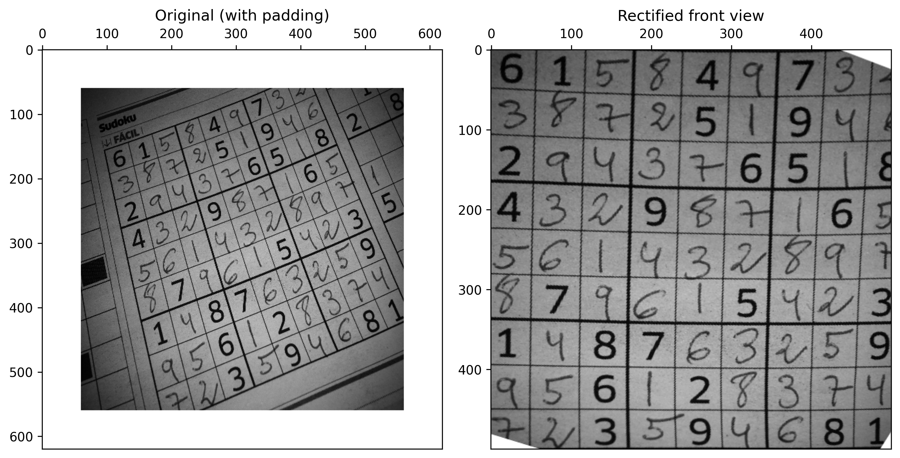
2.12.11 EP02_11 🏆 Perspective Correction (Homography) in a Real Image
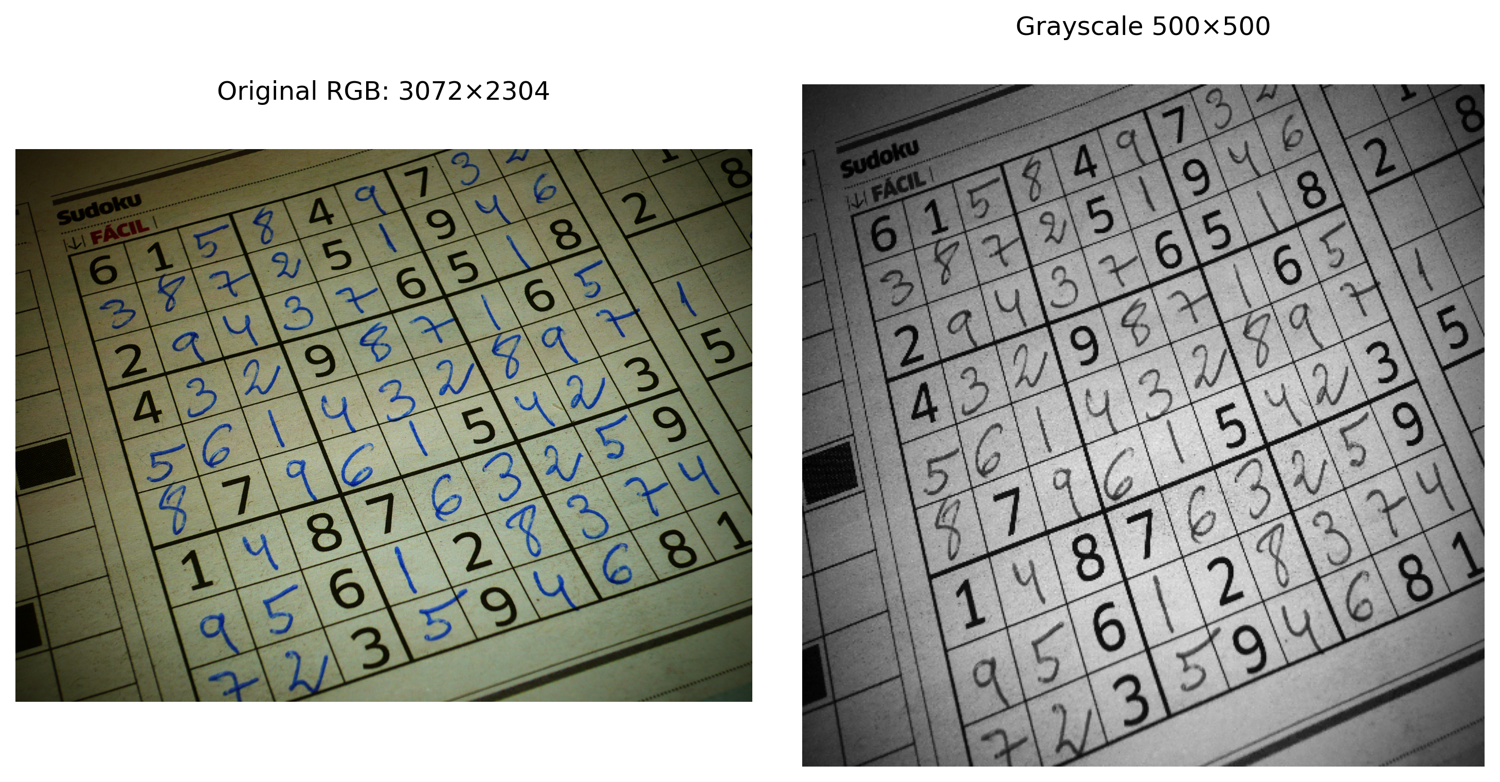
In this activity, the goal is to apply perspective transformation (homography) to “rectify” a tilted object in a real photograph. You will work with an image of a newspaper, where the grid of a Sudoku puzzle is distorted due to the angle at which the photo was taken.
Your program must read input parameters from the terminal, load the image, compute the \(3 \times 3\) homography matrix, apply the geometric transformation, and display a global validation indicator.
Read two integers L and C, representing the row and column dimensions (height and width) that the rectified output image should have.
Read four coordinate pairs\((x, y)\) from the terminal, representing the four corners of the source quadrilateral (the distorted Sudoku in the original image).
Automatically compute the four destination coordinate pairs using the provided dimensions \(L\) and \(C\), mapping the corners to the edges of the new image: \((0,0)\), \((C-1, 0)\), \((0, L-1)\), and \((C-1, L-1)\).
Load the local image sudoku.png and convert it to grayscale.
Compute the homography matrix and apply the spatial transformation to the image.
Output: Calculate and print the sum of all pixels of the resulting image.
📌 Important:
Input file: The image sudoku.png must be in the same folder as the script. The program must read it directly from disk (e.g., using mm.read("sudoku.png") or cv2.imread).
Point Order: Ensure that the reading of the 4 source points and the generation of the 4 destination points strictly follow the same corner order: Top-Left (TL), Top-Right (TR), Bottom-Left (BL), and Bottom-Right (BR).
Dimensions in OpenCV: Remember that functions such as cv2.warpPerspective expect the output image size in the format (width, height), which is equivalent to (C, L).
Interpolation: To ensure mathematical consistency of the pixel sum with the automatic grader, use the default bilinear interpolation (flags=cv2.INTER_LINEAR).
Credits: The image used is “Sudoku en periódico” by Héctor Rodríguez, licensed under CC BY 2.0.
2.12.11.1 🧠 Problem Context
The homography has 8 degrees of freedom, requiring at least 4 point correspondences to be computed. Unlike affine transformations, it maps any quadrilateral to another quadrilateral, allowing lines that converge to vanishing points to become parallel again:
Operation
Characteristic
Typical Application
Homography
Projection between planes
Document rectification, scanning of plates and QR Codes.
Inverse Mapping
Scanning from destination to source
Avoids “holes” or empty pixels in the final rectified image.
Warping
Spatial resampling
Correction of lens distortion and panorama stitching.
2.12.11.2 📌 Examples
Input
Output
Observation
500
500
100 120
420 95
80 440
450 460
32982820
The first two inputs are the output dimensions (\(L\) and \(C\)). The following 4 lines are the \((x, y)\) coordinates of the Sudoku corners in the original image + PAD. The output is the total sum of pixels of the rectified image.
200 200
100 120
420 95
80 440
450 460
5277150
Same source points as the previous example, but generating a smaller output image (\(200 \times 200\)). The pixel sum decreases proportionally due to the scale.
2.12.11.3 Sudoku image acquisition and conversion to grayscale
Figure 2.22 shows the reading of the original image followed by its conversion to grayscale and resizing to a \(500 \times 500\) pixel matrix, preparing the data for the next step.
The perspective correction, applied at Figure 2.23 via the homography matrix, eliminates distortions caused by the camera angle and produces a frontal, regular view of the Sudoku grid.
Figure 2.22: Acquisition of a Sudoku image on the left. On the right, conversion to grayscale and resizing. Credit: Héctor Rodríguez de Guardamar, Spain (CC BY 2.0).