9  Deep Learning for Computer Vision

The previous chapters established the foundations of Computer Vision (CV) through classical methods of feature extraction and representation. In Chapter 7, descriptors such as Local Binary Patterns (LBP) and Histogram of Oriented Gradients (HOG) showed how textures and shapes can be encoded by manually designed descriptors. In Chapter 8, algorithms such as Oriented FAST and Rotated BRIEF (ORB) and the Haar Cascade detector extended this principle to tasks of matching, detection, and object recognition.

These techniques remain relevant for their interpretability and computational efficiency, but they rely on a prior step of manually defining descriptors, known as feature engineering. This dependence limits the model’s adaptation to scenarios for which the descriptor was not designed.

Deep Learning proposes an alternative: instead of manually specifying the relevant features, the model automatically learns representations from the data during training—a process known as representation learning (GOODFELLOW, 2016). In CV, this strategy is implemented mainly through Convolutional Neural Networks (CNNs), in which convolutional filters no longer have fixed coefficients and are instead adjusted by optimization algorithms.

Although they represent a shift in the construction of pattern recognition systems, CNNs preserve concepts already studied in this book: the convolution, presented in Chapter 3, remains the operation responsible for local feature extraction, now applied with learned coefficients rather than designed ones.

It is worth noting that the goal of this chapter is not to exhaustively explore the theory of Deep Learning, but rather to offer an overview of its foundations and to demonstrate how these architectures are applied in the context of CV. Readers interested in a deeper theoretical and conceptual understanding of the field should refer to specialized references in the literature, such as Goodfellow (2016) and Lecun (2015).

9.1 Chapter Objectives

By the end of this chapter, the student should be able to:

• Relate the convolution learned by CNNs to the convolution of fixed kernels presented in Chapter 3;
• Describe the basic architecture of a CNN and the function of its main layers;
• Implement, train, and evaluate CNN models for image classification;
• Apply transfer learning to adapt pre-trained models to new problems;
• Use pre-trained models in classification, object detection, and segmentation tasks;
• Implement, train, and evaluate a U-Net architecture for semantic segmentation, comparing it to classical approaches;
• Prepare annotated datasets and integrate them into a training pipeline through platforms such as Roboflow;
• Integrate computational geometry and Deep Learning in augmented reality and photogrammetry applications.

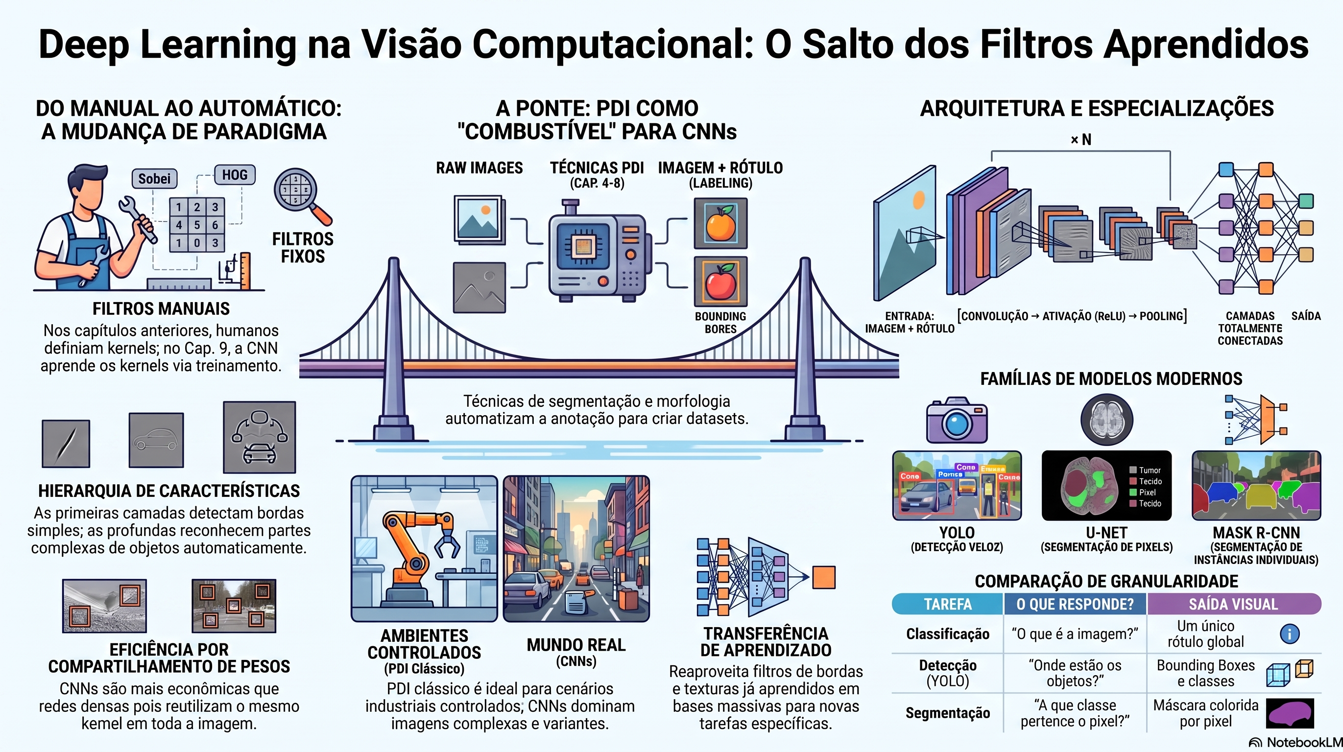
Figure 9.1 synthesizes the organization of the concepts studied in this chapter and the relationships among them.

Figure 9.1: Overview of the main concepts addressed in this chapter. Source: prepared with the aid of Gemini Notebook ({GOOGLE}, 2025).

9.2 Overview: Classification, Detection, and Segmentation

Computer vision tasks primarily differ in the information produced as output. Classification assigns a single label to the entire image; object detection locates and identifies objects present in the scene; segmentation associates a class with each pixel and, in some approaches, distinguishes different instances of the same category.

Table 9.1 summarizes the tasks studied throughout the book, indicating the question each one answers and the granularity of the information produced.

Table 9.1: Comparison among the main computer vision tasks according to the granularity of the information produced.

Task	Question Answered	Output Granularity	Chapter
Classification	“What is the class of this image?”	A single label for the entire image	7 and 9
Object detection	“Which objects exist and where are they?”	Class and bounding box for each object	8 and 9
Semantic segmentation	“To which class does each pixel belong?”	A class label for each pixel	8 and 9
Instance segmentation	“Which pixels belong to each object?”	One label per pixel for each instance	8 and 9
Panoptic segmentation	“What is the class and identity of each object?”	Class and instance identifier for each pixel	8 and 9

These tasks represent increasing levels of image interpretation: classification describes the scene globally, detection adds the location of objects, and segmentation produces a detailed spatial representation, allowing each region to be analyzed individually. This chapter focuses first on classification by CNNs, then extends the same principles to detection and segmentation.

9.3 Environment Setup

The examples in this chapter use PyTorch, a framework widely employed in the development and training of Deep Learning models. The following code checks the availability of the required libraries and automatically installs those not yet present in the execution environment.

If PyTorch is not installed, a version compatible with the available hardware is automatically selected: the version with CUDA support, if an NVIDIA GPU is available, or the CPU execution version, otherwise.

Next, the environment is initialized with the import of the libraries used throughout the chapter, the definition of a random seed to favor experiment reproducibility, and the retrieval of the morph.py file — the didactic morphological processing library already used in previous chapters —, if it is not yet available in the working directory.

import contextlib, importlib, importlib.metadata, importlib.util
import io, os, random, shutil, subprocess, sys, urllib.request, warnings

# Suppresses PyTorch warnings and general warnings
warnings.filterwarnings("ignore", category=UserWarning)

url = ("https://raw.githubusercontent.com/fzampirolli/"
       "pdi-vc/master/morph/config.py")
if not os.path.exists("config.py"):
    urllib.request.urlretrieve(url, "config.py")

import config

# Silences stdout and stderr both at Python level and at OS File Descriptor level
def setup_silencioso():
    with open(os.devnull, "w") as fnull:
        old_out = os.dup(1)
        old_err = os.dup(2)
        try:
            os.dup2(fnull.fileno(), 1)
            os.dup2(fnull.fileno(), 2)
            with contextlib.redirect_stdout(fnull), contextlib.redirect_stderr(fnull):
                config.setup()
        finally:
            os.dup2(old_out, 1)
            os.dup2(old_err, 2)
            os.close(old_out)
            os.close(old_err)

setup_silencioso()
from morph import mm


def setup_cap09():
    """Installs missing libs for this chapter in a 100% silent way."""
    pkgs = {
        "skimage": "scikit-image", "numpy": "numpy",
        "sklearn": "scikit-learn", "matplotlib": "matplotlib",
        "torchviz": "torchviz", "ultralytics": "ultralytics",
        "roboflow": "roboflow",
    }
    for mod, pkg in pkgs.items():
        if importlib.util.find_spec(mod) is None:
            subprocess.run([sys.executable, "-m", "pip", "install", "-q", pkg],
                           stdout=subprocess.DEVNULL, stderr=subprocess.DEVNULL)

    if importlib.util.find_spec("torch") is None:
        args = (["torch", "torchvision"] if shutil.which("nvidia-smi")
                 else ["--index-url",
                       "https://download.pytorch.org/whl/cpu",
                       "torch", "torchvision"])
        subprocess.run([sys.executable, "-m", "pip", "install", "-q", *args],
                       stdout=subprocess.DEVNULL, stderr=subprocess.DEVNULL)

    if not shutil.which("dot") and shutil.which("apt-get"):
        subprocess.run(["apt-get", "install", "-y", "-qq", "graphviz"],
                       stdout=subprocess.DEVNULL, stderr=subprocess.DEVNULL, check=False)


setup_cap09()

import cv2, numpy as np, torch
import torch.nn as nn
import torch.optim as optim
import matplotlib.pyplot as plt
import torchvision.models as models
import torchvision.transforms as T
from PIL import Image
from skimage import data as skdata
from sklearn.datasets import load_digits
from sklearn.model_selection import train_test_split
from torch.utils.data import DataLoader, TensorDataset
from torchvision.datasets import OxfordIIITPet
from torchvision.models.detection import (
    fasterrcnn_resnet50_fpn, FasterRCNN_ResNet50_FPN_Weights)
from torchvision.models.segmentation import deeplabv3_resnet50
from torchvision.transforms.functional import to_tensor
from torchviz import make_dot
from ultralytics import YOLO

torch.manual_seed(42)
FLAG_LIMPAR_DADOS = False
device = "cuda" if torch.cuda.is_available() else "cpu"
gpu = f" ({torch.cuda.get_device_name(0)})" if device == "cuda" else ""
ver = importlib.metadata.version("ultralytics")
print(f"✅ Environment ready. OpenCV {cv2.__version__} | "
      f"morph {getattr(mm, '__version__', 'local_file')} | "
      f"PyTorch {torch.__version__} | Ultralytics {ver} | {device}{gpu}")

✅ Environment ready. OpenCV 5.0.0 | morph local_file | PyTorch 2.6.0+cu124 | Ultralytics 8.4.113 | cuda (NVIDIA GeForce GTX TITAN X)

9.4 Fundamentals of Deep Learning for CV

CNNs are the primary Deep Learning architecture applied to image analysis. Their operation is based on the composition of convolutional operations organized into successive layers, in which the filters learned during training transform the image into progressively more abstract representations. This section presents the fundamental concepts that connect the spatial convolution studied previously to modern CV models, including hierarchical feature extraction, the training process, and the use of pre-trained models.

9.4.1 From Fixed Convolution to Learned Convolution

Chapter 3 presented spatial convolution with fixed kernels, such as the Sobel operators, designed to highlight specific features of an image. In Chapters 7 and 8, the same principle underpinned descriptors such as HOG, LBP, and ORB, as well as the Haar Cascade detector: in all these cases, the filters are defined before the execution of the algorithm and remain unchanged during processing.

Figure 9.2 revisits how spatial convolution works: the simulator allows selecting different kernels and following the displacement of the convolution window over an image. At each position, the kernel coefficients combine with the local neighborhood of the image — known as the receptive field — to produce a value in the feature map, also illustrating weight sharing.

CNNs preserve this operation but replace fixed kernels with learned filters: instead of predefined coefficients, the network adjusts these values during training from labeled examples, seeking to minimize a loss function, which measures the difference between the model’s predictions and the expected responses.

The essential difference between classical methods and CNNs, therefore, lies not in the convolution operation itself, but in how the filters are obtained: whereas the former use manually designed filters, CNNs learn, from the training data, representations suited to the task.

🎯 Simulator: Classic 2D Convolution Operation Input 12×12 · Kernel 3×3 · Stride 1

INPUT IMAGE (12×12)

FILTER (KERNEL 3×3)

Current Position: (0, 0) [Output 10×10]

Input (12×12)

Kernel (3×3)

Output Map (10×10)

∑ (xᵢ × wᵢ) = current position calculation...

Figure 9.2: Interactive simulator of classic 2D convolution: choose among the three synthetic 12×12 input images (house, happy or sad face) and a 3×3 filter (Sobel V, Sobel H, Sharpen, or Identity) and step forward to observe how the local inner products of the receptive field build the feature map cell by cell.

To understand how this learning occurs, it is necessary to study the basic processing unit of neural networks: the artificial neuron.

9.4.2 Artificial Neuron

The artificial neuron is the fundamental processing unit of a neural network. Its first mathematical model—a set of combined inputs compared against a threshold—was proposed by Mcculloch (1943), still without any learning mechanism. The Perceptron (ROSENBLATT, 1958) advanced this formulation by introducing a rule for adjusting weights based on examples, becoming the first artificial neuron model capable of learning and the foundation of modern Deep Learning architectures. The term Deep Learning refers to the use of networks with multiple processing layers, capable of learning hierarchical representations of data: the first layers learn simple features, such as edges and textures, and deeper layers progressively combine these representations to identify more complex structures and objects.

Each neuron receives a set of inputs, computes a linear combination of these values, and applies an activation function, producing a single output value. Mathematically, the linear combination is given by

\[ z=\sum_{i=1}^{n}w_i x_i+b, \]

where \(x_i\) represent the inputs, \(w_i\) the weights associated with each input, and \(b\) the bias. The neuron’s output is obtained by applying the activation function:

\[ y=f(z). \]

In CNNs, this principle assumes different forms depending on the layer. In convolutional layers, each neuron processes only a small region of the input, called the receptive field, preserving the spatial organization of the image. In fully connected layers, each neuron receives all outputs from the previous layer, combining the extracted features to produce the network’s final output, such as the class assigned to the image.

Figure 9.3 illustrates the functioning of an artificial neuron: the simulator allows modifying the inputs (\(x_1\) and \(x_2\)), the weights (\(w_1\) and \(w_2\)), the bias (\(b\)), and the activation function, observing in real time the calculation of the linear combination and the corresponding output.

⚙️ Simulator: Artificial Neuron in a CNN y = f(∑ wᵢxᵢ + b)

Pixel x₁ (normalized) / Kernel weight w₁

x₁ w₁

Pixel x₂ (normalized) / Kernel weight w₂

x₂ w₂

Bias (b) and Function f(z)

b ReLU Sigmoid Step Identity

The values of x range from -3 to 3 because, in a CNN, pixels (0–255) are normalized before entering the network. The drawing on the side translates that normalized value back into a gray tone, just for visual intuition — the numbers that count for the calculation are the ones on the bars.

Receptive Field → Convolution → Feature Map

Activation at f(z)

x₁, x₂ = intensity of pixels in the receptive field · w₁, w₂ = kernel (filter) weights · z = convolution result at this position · y = pixel value produced in the feature map, after activation.

z = (1.00 × 0.80) + (-1.50 × 0.50) + 0.20 = 0.25 → y = 0.25

Figure 9.3: Interactive simulator of the Artificial Neuron in a CNN context: toggle between a convolutional layer neuron (where x_i are pixel intensities in a receptive field and w_i are kernel weights) and a fully connected layer neuron, adjusting inputs, weights, bias, and activation function to visualize the computation of z and output y in real time.

In a CNN, thousands of neurons are organized into layers with specific functions: the first ones are responsible for feature extraction through convolution, and the last ones perform classification based on the learned features.

9.4.3 Convolutional Layer

The convolutional layer is responsible for extracting features from the image. Each filter generates a feature map, whose intensity at each position indicates the filter’s response to the corresponding region of the input.

The operation performed follows the same principle of shifting and local combination presented in Chapter 3 for spatial convolution. Considering a kernel \(K\) of dimension \(k \times k\), the value produced at position \((i,j)\) is given by

\[ F(i,j)=\sum_{u=0}^{k-1}\sum_{v=0}^{k-1}K(u,v)\,I(i+u,j+v). \]

It is worth noting a terminological distinction: the expression above formally corresponds to a cross-correlation, rather than strict mathematical convolution, which requires reflecting the kernel before combination. Most Deep Learning frameworks, including PyTorch, implement this operation without reflection and designate it, by convention, as convolution — a convention also adopted in this chapter. This difference has no practical effect on training, since the kernel coefficients are learned rather than imposed beforehand.

The main difference from classical methods therefore lies in obtaining the kernel \(K\): in traditional filters, its coefficients are manually defined to highlight specific image features; in CNNs, the coefficients are initialized automatically and adjusted during training through error backpropagation, making each filter specialized in identifying patterns relevant to the task under study.

Two concepts characterize this layer:

• Weight sharing: the same filter is applied at all positions of the image, significantly reducing the number of model parameters.
• Receptive field: each convolutional neuron processes only a small neighborhood of the image, preserving the spatial structure of the data.

By stacking multiple convolutional layers, the network learns a feature hierarchy: the early layers tend to detect simple patterns, such as edges and textures, and the deeper layers combine this information to represent progressively more complex structures. After convolution, the feature map is subjected to an activation function, introducing nonlinearity into the model and expanding its capacity to represent complex relationships among input variables.

Figure 9.4 presents this layer interactively.

⚙️ Simulador: Operação de Convolução & Mapa de Características F(i,j) = f(∑ K(u,v) · I(i+u, j+v))

IMAGEM DE ENTRADA

KERNEL (FILTRO FIXO)

Posição do Campo Receptivo

Função de Ativação f(z)

ReLU Identidade (Linear) Sigmoide

Preenchimento (Padding)

Zero-Padding (p = 1)

pixel real margem fixa da imagem (0) padding do algoritmo (0)

O mesmo kernel desliza sobre toda a imagem reutilizando seus coeficientes (compartilhamento de pesos). Cada imagem já vem cercada por uma margem fixa de 1 pixel de fundo (zeros, contorno tracejado âmbar), isolando a forma nos quatro lados. Escolha uma imagem e um kernel fixo acima, depois use ◀ ▶ ou "Auto" para percorrer o campo receptivo — o Feature Map à direita é preenchido célula a célula, na mesma ordem em que a convolução é calculada (as células ainda não visitadas aparecem como "···").

📌 A saída F(i,j) vem do campo receptivo entre (i,j) e (i+2,j+2); seu centro real é (i+1,j+1) — 1 linha e 1 coluna abaixo/à direita do índice usado para rotular a célula, sempre nas duas direções. Esse deslocamento só fica visível no eixo em que o kernel diferencia a imagem (por isso o Sobel V parece deslocar só para o lado, e o Sobel H, só para baixo).

Ativação em f(z)

🔍 Cálculo Detalhado no Campo Receptivo Atual

z = 0.00 → y = ReLU(z) = 0.00

Figure 9.4: Interactive Convolutional Layer Simulator: choose among three 12×12 input images (house, happy face, or sad face) to observe how the same fixed kernels react to different edges and shapes. Navigate the receptive field with the buttons or automatic playback, adjust the activation function and toggle zero-padding, while the feature map is revealed cell by cell, with detailed term-by-term calculation and the output dimension formula in real time.

9.4.4 Activation Function

Convolution is a linear operation. To enable the network to model nonlinear relationships between inputs and outputs, an activation function is applied after each convolutional layer.

The most commonly used function in CNNs is ReLU (Rectified Linear Unit), defined as

\[ \mathrm{ReLU}(x)=\max(0,x). \]

This function preserves positive values and replaces negative values with zero, introducing nonlinearity into the model and facilitating the training of deep networks at low computational cost.

Figure 9.5 illustrates the behavior of ReLU applied to both individual values and a feature map, allowing a comparison of the output before and after activation.

⚡ Simulator: ReLU Activation Function ReLU(x) = max(0, x)

x = x = -2.50 → ReLU(x) = 0.00

ReLU function curve

Feature map: before / after

Figure 9.5: Interactive simulator of the ReLU activation function: drag the control to see how negative values are zeroed out and positive values are preserved, both in the curve and in a real feature map.

The feature maps resulting from convolution and activation preserve the spatial structure of the image. In many architectures, the next step reduces their resolution through a pooling operation.

9.4.5 Pooling

The pooling layer reduces the spatial resolution of feature maps while preserving the most relevant information for subsequent processing stages. The most commonly used operation is max-pooling, which selects the largest value within each window of the image:

\[ P(i,j)=\max_{(u,v)\in\text{window}(i,j)}F(u,v). \]

This reduction lowers the computational cost of subsequent layers and makes the representation more robust to small variations in the position of patterns present in the image.

Figure 9.6 illustrates this operation on an 8×8 pixel feature map, reduced to 4×4 using 2×2 windows with a stride of 2, alternating between max-pooling and average-pooling — which, instead of the maximum, computes the average of the values within the corresponding window.

🔻 Simulator: Pooling 2×2 window, stride 2

Type:

Current window: (0, 0) of 4×4

O max-pooling only retains the largest value from each 2×2 window, halving the spatial resolution and preserving the strongest responses of the feature map.

Input map (8×8) — current window highlighted

Reduced map (4×4)

Figure 9.6: Interactive pooling simulator: choose between max-pooling and average-pooling and step forward to observe the reduction of the spatial resolution of the feature map.

Together, convolution, activation function, and pooling form the basic building block used in constructing a CNN.

9.4.6 Training Neural Networks: How CNNs Learn

A CNN learns by automatically adjusting its parameters — the coefficients of the convolutional filters, the weights of the fully connected layers, and the biases (biases) — from labeled examples. This training is iterative and involves three steps: measuring the error produced by the network through a loss function, calculating how this error depends on each parameter through backpropagation, and updating the parameters with an optimization algorithm (optimizer).

9.4.6.1 Loss Function

The loss function quantifies the difference between the network’s prediction and the correct answer, referred to as the ground truth. The result is a scalar \(L\): the lower the loss, the closer the prediction is to the expected answer.

In multiclass classification problems, the most commonly used function is Cross-Entropy Loss, applied to the probabilities produced by the Softmax layer:

\[ L=-\sum_{c=1}^{C} y_c \log(\hat{y}_c), \]

where \(C\) is the number of classes, \(y_c\) is the actual label in one-hot encoding, and \(\hat{y}_c\) is the predicted probability for class \(c\). The loss approaches zero when the network assigns high probability to the correct class and grows rapidly as that probability decreases.

Figure 9.7 illustrates this behavior: the simulator allows selecting the correct class and altering the probabilities produced by Softmax, showing in real time the variation of the loss function.

📉 Simulator: Loss Function (Cross Entropy) L = -log(ŷ_target)

THE IMAGE'S ACTUAL CLASS (GROUND TRUTH: y_c = 1)

PROBABILITIES ESTIMATED BY SOFTMAX (ŷ_c)

🏠 House (ŷ_1): 0.70

😊 Happy (ŷ_2): 0.20

😢 Sad (ŷ_3): 0.10

Penalty Curve L = -log(ŷ_target)

LOSS CALCULATION:

Loss L = 0.3567

Figure 9.7: Interactive simulator of the Loss Function (Cross-Entropy): select the real class of the image (House, Happy or Sad) and adjust the probabilities estimated by Softmax to visualize the calculation of the scalar penalty and the graph of the negative logarithm in real time.

9.4.6.2 Backpropagation

After computing the loss, it is necessary to determine how each network parameter contributes to this result. This step is carried out by backpropagation, which applies the Chain Rule of differential calculus to obtain the gradient of the loss function with respect to each parameter.

For a parameter \(w\), this gradient is given by

\[ \frac{\partial L}{\partial w}. \]

The gradient indicates how the loss varies with respect to small changes in \(w\): a positive gradient indicates that increasing \(w\) increases the loss, and a negative gradient indicates the opposite effect.

Figure 9.8 presents this process visually, showing the propagation of the gradient from the output layer to the earliest convolutional layers.

⬅️ Simulator: Backpropagation ∂L/∂w = (∂L/∂y) · (∂y/∂z) · (∂z/∂w)

Step 1 of 4: Output (Loss & Softmax)

ERROR PROPAGATION DIRECTION (REVERSE FLOW ⟵)

Conv1 Kernels

∂L/∂K

⟵

Max-Pooling

∂L/∂X_pool

⟵

FC Layers

∂L/∂W_fc

⟵

Loss / Softmax

∂L/∂y_pred

🔗 Chain Rule in Current Layer:

Figure 9.8: Interactive Backpropagation simulator: advance through the Chain Rule steps to follow the error signal flow in the reverse direction of the network, observing the computation of partial derivatives of the gradient at each layer.

9.4.6.3 Optimization Algorithms

After computing the gradients, an optimization algorithm (optimizer) updates the network parameters to reduce the loss function. In deep networks, this search occurs in a high-dimensional space and, in general, a non-convex one, which makes optimization a challenging problem.

To facilitate understanding, Figure 9.9 uses a simplified loss surface, with a global minimum, a local minimum, and a barrier between these regions. The global minimum corresponds to the smallest value of the loss function and represents the best set of network parameters; a local minimum also exhibits low loss but may be far from the best solution. When optimization becomes trapped in a local minimum, the adjustments to filters, weights, and biases become very small, and training stops before reaching a model with lower error.

9.4.6.3.1 Stochastic Gradient Descent (SGD)

Stochastic Gradient Descent (SGD) updates the parameters in the opposite direction of the gradient:

\[ w_{\text{new}} = w_{\text{current}} - \eta \frac{\partial L}{\partial w}, \]

where \(\eta\) is the learning rate, responsible for controlling the size of the update. SGD uses only the gradient of the current iteration; when the search reaches a local minimum, the gradients become very small and updates practically cease.

9.4.6.3.2 Adaptive Optimizers: Adam

Adam (Adaptive Moment Estimation) combines adaptive estimates of the first and second moments of the gradients (KINGMA, 2015), adjusting the learning rate for each parameter individually. In many cases, this adaptation helps overcome local minima that would trap SGD.

Figure 9.9 compares the trajectory of SGD and Adam over the same non-convex loss surface.

⚡ Simulator: Optimization with Contour Lines (SGD vs. Adam) Non-Convex Terrain: Local vs. Global Minimum

💡 How to read this map: a yellow arrow points in the direction of descent (−∇L), which is the opposite of the gradient vector (∇L). The optimizer moves in this direction to reduce the loss L(w₁, w₂) until reaching the deepest regions (darker shades).

MAIN ALGORITHM (solid line)

LEARNING RATE (η)

0.12 (High) 0.05 (Ideal) 0.01 (Slow)

👻 Show ghost trajectory of the other optimizer (instant comparison)

Loss Heatmap L(w₁, w₂) — click to choose the start

Global Minimum Local Minimum Gradient (↓ descent) Main trajectory Ghost (other optimizer)

OPTIMIZATION STATE:

w₁ = 1.80, w₂ = 0.20

Loss L = 2.450

STEP

0

|∇L| (MAGNITUDE)

0.000

Status: Starting Point

Figure 9.9: Interactive simulator of Optimization Algorithms: compare the trajectory of SGD and Adam over a non-convex loss surface with a heatmap and contour lines. The solid line shows the selected optimizer advancing step by step; the dashed line shows, for instant comparison, the full path that the other optimizer would take from the same starting point. Notice how SGD gets stuck in the Local Minimum on the right, while Adam may or may not cross the central barrier depending on accumulated momentum and learning rate. Click anywhere on the plot to reset the starting point of the weights.

9.4.7 Architecture of a CNN

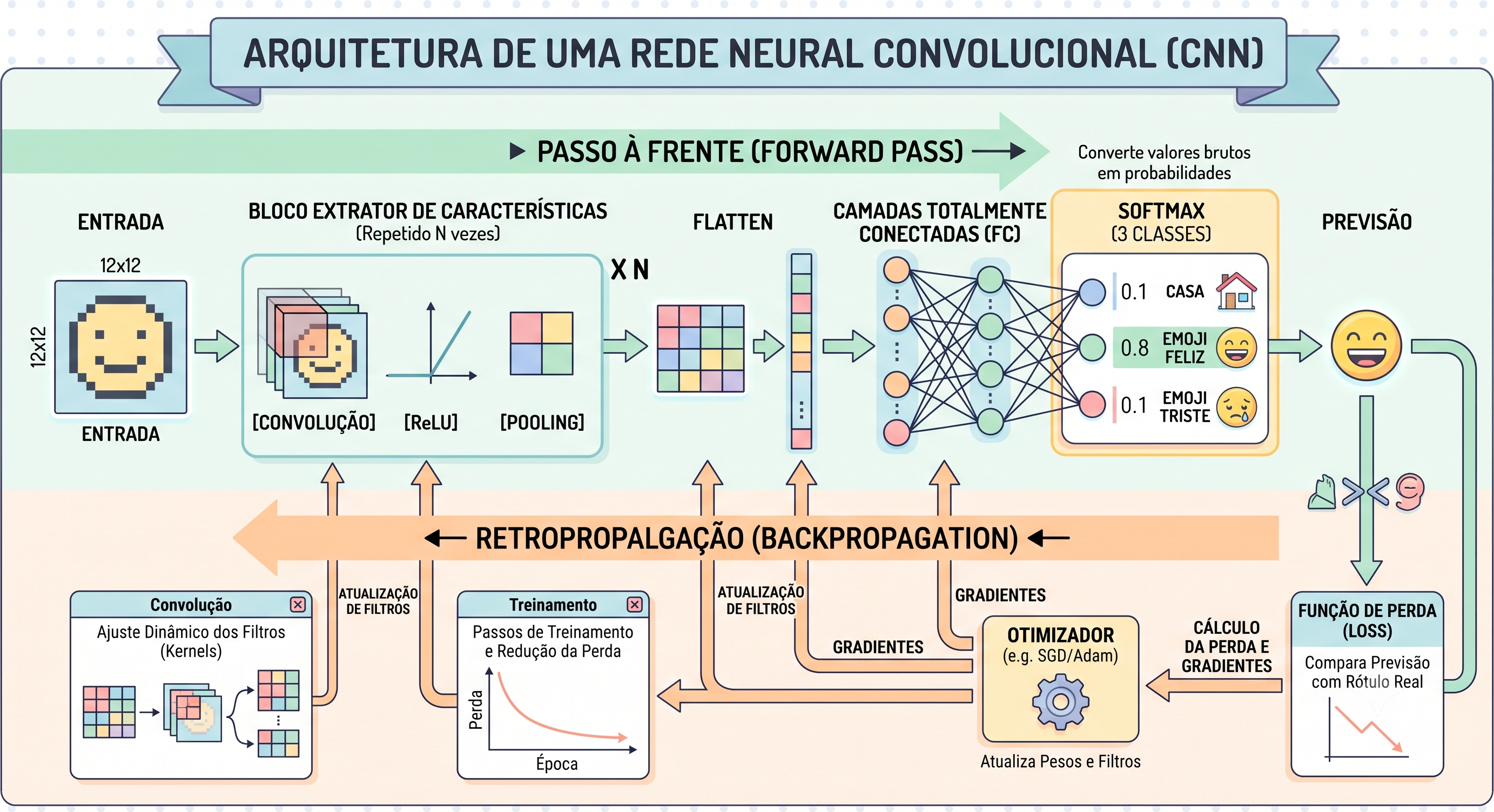
A CNN for image classification combines the layers presented in the previous sections. During the forward pass, the image successively traverses the convolutional layers, the activation functions, the pooling operations, the Flatten step, the fully connected layers, and finally the Softmax layer, which produces the class probabilities. During training, this prediction is compared to the correct label to compute the loss function, perform backpropagation, and update the parameters through an optimization algorithm.

Figure 9.10 presents this processing and training flow.

Figure 9.10: Simplified architecture of a CNN for image classification, highlighting the forward pass and the training steps through the loss function, backpropagation, and the optimization algorithm.

After the last convolutional block, the Flatten operation reorganizes the feature maps into a one-dimensional vector, which feeds the fully connected layers, responsible for combining the extracted features to produce the scores (logits) for each class. The Softmax layer converts these scores into a probability distribution, used both for classification and for computing the loss function during training.

Figure 9.11 presents an interactive version of this architecture, allowing successive training steps to be executed and enabling observation of the loss reduction, the backpropagation of gradients, and the update of the network filters.

⚙️ Simulator: Full CNN Architecture Input (12×12) → Conv → Pool → FC → Softmax

PIPELINE INPUT IMAGE (12×12)

🎯 Training (Forward Pass + Backpropagation)

Input ▸ Conv+ReLU ▸ Pool ▸ Flatten ▸ FC ▸ Softmax ▸ Prediction

Loss ◂ Optimizer ◂ Backpropagation ◂ (each step)

LOSS

ACCURACY

Loss: —

Accuracy: —

Training step: 0

The kernels and weights start random (no longer the fixed filters of the previous simulator). Each step, the network does the forward pass on the 3 images, computes the loss (cross-entropy) e a accuracy (how many of the 3 images are classified correctly), backpropagates the error, and adjusts all weights (including the kernels of the convolution) via gradient descent. ⚠️ Since the "training set" has only 3 examples, this demonstrates the mechanism of training (loss decreasing, accuracy increasing, weights changing) — not the ability to generalize to new images, which would require much more data.

Figure 9.11: Interactive simulator of a CNN architecture: choose one of the 12×12 input images (house, happy face, or sad face), click on each block of the pipeline — Input, Conv+ReLU, Pooling, Flatten, FC, and Softmax — and run real training steps (forward pass + backpropagation) to observe the loss and accuracy evolving, the kernels being adjusted, and the Softmax starting to point to the correct class.

9.4.8 How the Gradient Adjusts Convolution Kernels

Understanding the learning process in a Convolutional Neural Network (CNN) requires elucidating a fundamental mechanism: how the random coefficients of an initial filter transform into precise detectors of edges, textures, and complex patterns.

The answer lies in the principle of weight sharing. During the forward pass, the same filter of dimension \(3\times3\) slides across the entire extent of the input image. Consequently, each kernel weight—such as the element \(K[0][0]\) in the upper-left corner—is reused multiple times across the different spatial regions of the input data.

During backpropagation, this reuse establishes a direct dynamic: each spatial position processed by the filter generates an individual contribution (“vote”) for the update of the respective weight.

9.4.8.1 The Intuition Behind the Calculation

Let \(Z[r][c]\) be the pre-activation feature map at position \((r,c)\) of the sliding window, obtained by the cross-correlation between the kernel \(K\) and the input \(X\):

\[ Z[r][c] = \sum_{k_r} \sum_{k_c} K[k_r][k_c] \cdot X[r + k_r][c + k_c] \]

Applying the chain rule to determine the contribution of a specific weight \(K[k_r][k_c]\) to the loss function \(L\), the following steps are obtained:

1. Local Error (\(dZ\)): At each position \((r,c)\), the partial derivative of the loss function with respect to the pre-activation is computed: \[dZ[r][c] = \frac{\partial L}{\partial Z[r][c]}\] which quantifies the responsibility of that specific position for the total network error (\(L\)).

2. Weight Contribution: Since \(\frac{\partial Z[r][c]}{\partial K[k_r][k_c]} = X[r + k_r][c + k_c]\), the influence of a specific weight \(K[k_r][k_c]\) on the error at position \((r,c)\) is obtained by multiplying the local error \(dZ[r][c]\) by the value of the input pixel aligned with that weight at the time of the computation: \[dZ[r][c] \cdot X[r + k_r][c + k_c]\]

3. Gradient Accumulation: The final gradient of the weight corresponds to the sum of the contributions (“votes”) from all positions traversed by the sliding window:

\[ \frac{\partial L}{\partial K[k_r][k_c]} = \sum_{(r,c)} dZ[r][c] \cdot X[r + k_r][c + k_c] \]

This formulation ensures direct parity between the analytical derivation and the values computed in the gradient inspection simulator (Figure 9.12).

9.4.8.2 The Role of the ReLU Function as a “Relevance Filter”

The application of the ReLU activation function (\(\max(0, z)\)) immediately after the convolution introduces a selectivity property to the gradient:

• Positive Activation (\(Z[r][c] > 0\)): The derivative of ReLU is \(1\). The local error is propagated in full (\(dZ \neq 0\)), allowing the position to contribute to the kernel weight updates.
• Inactive Activation (\(Z[r][c] \le 0\)): The derivative of ReLU is \(0\). The local error is nullified (\(dZ = 0\)), suppressing the position’s contribution to the final gradient.

Pedagogical note: ReLU ensures that only the spatial regions that produced active responses during the forward pass have the ability to modify the kernel weights in the backpropagation process.

9.4.8.3 Weight Update via Gradient Descent

After consolidating the accumulated gradients from all positions, the weight update occurs according to the Stochastic Gradient Descent (SGD) algorithm:

\[ K[k_r][k_c] \leftarrow K[k_r][k_c] - \eta \cdot \frac{\partial L}{\partial K[k_r][k_c]} \]

where \(\eta\) denotes the learning rate.

• If the sum of the gradients is positive, the weight value is reduced.
• If the sum is negative, the weight value is increased.

9.4.8.4 Exploring the Interactive Simulator

Note🔗 From Global Architecture to Gradient Inspection

In the architecture simulator (Figure 9.11), one observes the error \(dZ\) derived from the complete multilayer backpropagation, originating from the softmax cross-entropy loss over the \(12\times12\) input images.

To enable the analytical verification of the gradient without the overhead of \(100\) convolution positions and multilayer backpropagation, the kernel learning simulator (Figure 9.12) adopts a reduced inspection model (\(6\times6\)). In this scenario, the problem is simplified by replacing the complex classification with a scalar calibration target: the filter is adjusted to produce a predefined accumulated response (\(\text{target} = 9\)) when identifying a specific pattern (such as a 45-degree edge). The gradient accumulation mechanism (\(dZ \cdot X\)) remains strictly identical in both formulations.

To inspect this dynamic at the numerical level, use the simulator in Figure 9.12:

• Input Image (\(X\)): \(6\times6\) matrix.
• Convolutional Filter (\(K\)): \(3\times3\) matrix (9 weights).
• Output Map (\(Z\) / \(A\)): \(4\times4\) matrix (16 window positions).
• Loss Function (\(L\)): Defined by \(L = \frac{1}{2}(S - \text{target})^2\), where \(S = \sum A[r][c]\) represents the global sum of post-ReLU activations.

The role of \(\text{target} = 9\): The scalar value \(\text{target} = 9\) represents the ideal “activation energy” stipulated for the image with a diagonal edge. Since the map \(A\) has 16 positions, this value is equivalent to seeking an average response of \(\frac{9}{16} \approx 0.56\) per activated pixel. When \(S > 9\), the network identifies that the filter is reacting with excessive intensity to the pattern, generating an error \(dZ > 0\) that forces a reduction in the weights \(K\). When \(S < 9\), the weights are increased to amplify the signal.

9.4.8.4.1 Suggested Experimentation Script:

1. Weight Selection: In the \(3\times3\) grid, choose the weight to be analyzed (e.g., \(K[0][0]\)).
2. Window Scan: Use the “▶ Advance position” button to track the window’s displacement across the 16 spatial positions. Note the visual highlight on the input map cell that aligns the pixel \(X\) with the selected weight.
3. Local Vote Analysis: Examine the product of the local error and the input pixel (\(dZ \cdot X\)) in the position calculation panel.
4. History Verification: Track the consolidation of the 16 partial results organized in the four history columns, observing the accumulation of the final gradient.
5. Kernel Update: Click on “▶ Apply gradient descent step” to visualize the convergence of the loss curve and the adaptation of the random kernel to the selected input pattern.

🧮 Simulator: Kernel Weight Gradient ∂Loss / ∂K[kr][kc] = Σ dZ · X

INPUT PATTERN (IMAGE 6×6)? Choose which image 6×6 feeds the convolution.

LEARNING RATE (η)? Learning rate. Adjust to see the difference between smooth convergence (0.002) and collapse from overshooting (0.02).

Example reduced: image 6×6 and filter 3×3 generating maps 4×4. Click the tabs "🔍 How is it calculated?" below each matrix to understand the calculations step by step. Hover over any cell in X, Z, A, dZ, or K to see the exact calculation for that value, with the elements used in the related layers highlighted with a dashed/blue outline.

1. KERNEL WEIGHT? Select which kernel weight you want to analyze individually.

CURRENT KERNEL (K)? Filter 3×3 values. The selected weight is highlighted in blue. Hover over a weight to see where it is used.

🔍 How is it updated?

Gradient Rule:

K ← K − η · ∇K

• η = learning rate.
• ∇K = sum of the 16 dZ votes × X.

INPUT X (6×6)? Image 6×6. Blue pixel = overlap with the selected kernel weight K in the current window. Hover over a pixel to see which Z positions it is used in.

🔍 How does X work?

Input matrix. At position (r,c), weight K multiplies the pixel:

X[r + k_r][c + k_c]

PRE-ACTIVATION Z (4×4)? Convolution result before ReLU: Z = Σ K · X. Hover over a cell to see the 9 terms of the sum, highlighting the window in X and the entire kernel K.

🔍 How is Z calculated?

Cross-correlation:
Pointwise multiplication of filter 3×3 over X:

Z[r][c] = Σ K · X

ACTIVATION A (4×4)? Post-ReLU result: A = max(0, Z). If Z ≤ 0, the activation is zeroed. Hover over a cell to highlight the corresponding Z.

🔍 How is A calculated?

ReLU function:

A[r][c] = max(0, Z[r][c])

Global Sum (S):

S = Σ A[r][c]

ERROR dZ (4×4)? Propagated error: dZ = (S - target) · I(Z > 0). Where A=0, the error dZ is also 0. Hover over a cell to see the full calculation, highlighting the corresponding Z and all 16 cells of A that form S.

🔍 How are dZ, S, and Loss calculated?

1. Loss (Loss L):

L = ½ (S − target)²

2. Propagated error dZ:

dZ = (S − target) · deriv_ReLU(Z)

2. CALCULATION AND SUM OF EACH POSITION'S "VOTES"? Each position (r,c) generates a vote = dZ[r][c] × X[r+kr][c+kc]. The sum of all 16 votes forms the weight gradient.

CALCULATION OF THIS POSITION? Displays the local error (dZ) and input pixel (X) multiplied at the current sliding window position.

ACCUMULATED SUM (GRADIENT)? The accumulated value of the products dZ × X from all positions already visited. When it reaches 16/16, this is the final weight gradient.

HISTORY OF THE 16 POSITIONS (COLUMNS c=0, c=1, c=2, c=3)? Follow the list of all 16 positions organized in 4 columns to match the window movement over the output image.

3. USE THE GRADIENT TO UPDATE THE KERNEL? Applies the Gradient Descent rule (K ← K − η · gradient) to all 9 weights.

LOSS OVER UPDATES? Evolution of error L = ½(S − target)²:
• Objective: L → 0 (S → target).
• If stuck at L = 40.5: "Overshooting" occurred (exaggerated leap). The weights became very negative, generating Z ≤ 0 (ReLU death). With S = 0, the loss freezes at ½(0 − 9)² = 40.5.

Figure 9.12: Interactive simulator for computing the gradient of a weight from the convolutional kernel.

Note🧠 Synthesis — From convolution to representation learning

The simulators in this section demonstrate, in a sequential manner, how a CNN transforms an input image into a probabilistic estimate and how its parameters are optimized during training:

• Convolution: applies filters to the image to extract local features, generating feature maps through weight sharing.
• ReLU: introduces nonlinearity into the system, enabling the modeling of complex relationships among data.
• Pooling: reduces the spatial resolution of the feature maps, decreasing computational cost and conferring invariance to small local translations.
• Flatten: reorganizes the multidimensional maps into a one-dimensional vector for feeding subsequent layers.
• Fully connected layer: combines the extracted features to produce raw scores (logits) associated with each class.
• Softmax: converts the logits into a normalized probability distribution.
• Loss function: compares the predicted distribution with the ground truth, quantifying the network’s error as a scalar.
• Backpropagation: applies the chain rule to compute the partial derivative (gradient) of the loss function with respect to each trainable parameter.
• Optimizer: updates the coefficients of filters, weights, and biases in the direction opposite to the gradient, reducing the loss at each iteration.

Throughout the iterations, the convolutional filters evolve from stochastic values into specialized detectors: early layers learn low-level visual primitives (such as edges and textures), while deeper layers consolidate these representations into abstract and semantic structures.

9.5 Practical Applications in CV

After the theoretical consolidation of the fundamentals of CNNs and the visual verification of each of their elementary operations through interactive simulators, it becomes essential to observe the integration of these steps into complete programming pipelines.

In the following sections, the theory is translated into executable code in PyTorch, exploring the three fundamental tasks of CV: classification, object detection, and semantic segmentation. This practical progression allows for analysis ranging from the construction of a convolutional architecture trained from scratch to the application of advanced transfer learning strategies in pre-trained models for synthetic and real datasets.

9.5.1 Image Classification with CNNs

Image classification is one of the most traditional applications of CNNs. In this task, the goal is to assign a single label to the input image, such as identifying an object category, an animal species, or a diagnostic class. To achieve this, the CNN progressively transforms pixel values into higher-level abstract representations, combining convolutional layers, activation functions, and spatial reduction operations until it produces a probability distribution across the possible classes. In this section, we present the basic architecture of a classifying CNN, the data transformation flow along the network, and the training process for adjusting the learned parameters.

9.5.1.1 Training a CNN from Scratch on Digits

To establish a direct comparison with the approaches presented in Chapter 7, this section develops a CNN trained on the same handwritten digits dataset (load_digits). The fundamental difference lies in the representation step: while classical methods rely on raw pixels or manually calculated descriptors, such as the Histogram of Oriented Gradients (HOG), the CNN automatically learns the coefficients of the convolutional filters during the optimization process.

The following codes (consolidated in Figure 9.15) carry out data preparation, define a simple convolutional architecture in PyTorch, execute the training loop using the Adam algorithm, and generate the evolution curves of the loss function and accuracy.

9.5.1.1.1 Block 1: Data Preparation and Structuring

The initial stage of any Deep Learning pipeline consists of converting and adapting the input data to the format required by the scientific computing framework.

9.5.1.1.1.1 The Concept of Tensor

In Deep Learning, the fundamental data structure is the tensor. From a computational perspective, a tensor consists of a multidimensional array of numbers generalized to \(n\) dimensions:

• A 0th-order tensor is a scalar (a single value).
• A 1st-order tensor is a vector (length).
• A 2nd-order tensor is a matrix (rows and columns).
• A 3rd-order or higher tensor represents a volume or hyper-array of data.

In the context of PyTorch, the torch.Tensor class extends the functionality of multidimensional numerical arrays (such as those in NumPy) by offering support for hardware-accelerated operations via GPUs (Graphics Processing Units) and support for automatic derivative computation (autograd), which is essential for the backpropagation algorithm.

9.5.1.1.1.2 Analysis of the Preprocessing Code

1. Loading and Normalizing Intensities: The load_digits dataset contains \(1,797\) samples of handwritten digits of \(8 \times 8\) pixels, whose original intensities range on the integer scale from \(0\) to \(16\). Dividing by \(16.0\) performs the normalization of the data to the range \([0.0, 1.0]\). This floating-point scaling transformation (float32) is indispensable in neural networks to prevent saturation of activation functions and to stabilize the computation of gradients in the optimization algorithm.

2. Stratified Split (70% Training / 30% Testing): The train_test_split function separates \(70\%\) of the samples for adjusting the network parameters and reserves \(30\%\) for evaluating the model on unseen data. The stratify=y parameter ensures stratified sampling, maintaining the exact proportion of each of the 10 digit classes (\(0\) to \(9\)) in both sets, thereby preventing distribution bias.

3. Dimensional Adaptation for 2D Convolution (unsqueeze): In CNNs, two-dimensional convolutional layers (nn.Conv2d) require that the input tensor strictly possess 4 dimensions in the ordering \((N, C, H, W)\):

   • \(N\): number of samples (batch size).
   • \(C\): number of color channels (\(1\) for grayscale, \(3\) for RGB).
   • \(H\): image height in pixels (\(8\)).
   • \(W\): image width in pixels (\(8\)).

   Since the original array has a \(3\text{D}\) shape of the type \((N, 8, 8)\), the call .unsqueeze(1) inserts a singleton dimension specifically at index 1 (the position reserved for the color channel \(C\)), transforming the structure into a \(4\text{D}\) tensor of shape \((N, 1, 8, 8)\), as required by PyTorch.

4. Label Conversion (dtype=torch.long): The class labels \(y\) are converted into 64-bit integer tensors (torch.long). This type specification is a requirement of the Cross-Entropy loss function (nn.CrossEntropyLoss), which uses non-negative integers as indices to associate the correct class with the network’s output logits.

Attention to Dimensions: The final structure is represented by the tensor (N, 1, 8, 8), where N is the number of samples (batch size), 1 is the color channel (grayscale), and 8×8 is the spatial resolution of the image in pixels.

Figure 9.13 illustrates a sequence of samples from the training set after preprocessing and dimensional adaptation to PyTorch tensors. In the display step, the call img.squeeze().numpy() chains two transformations: the .squeeze() method eliminates the redundant singleton dimension of the color channel, reducing the \(3\text{D}\) tensor of shape (1, 8, 8) to a \(2\text{D}\) matrix of (8, 8); subsequently, the .numpy() method converts the PyTorch structure into a native NumPy array, a format required by graphical rendering tools such as mm.show().

# 1. Data loading and preprocessing
digits = load_digits()
X = digits.images.astype(np.float32) / 16.0  # Normalization to the range [0, 1]
y = digits.target

# Stratified split into training (70%) and test (30%) sets
X_treino, X_teste, y_treino, y_teste = train_test_split(
    X, y, test_size=0.3, random_state=42, stratify=y
)

# Adjusting to the dimension expected by PyTorch: (N_samples, Channels, Height, Width)
X_treino_t = torch.tensor(X_treino).unsqueeze(1)   # Dimension: (N, 1, 8, 8)
y_treino_t = torch.tensor(y_treino, dtype=torch.long)
X_teste_t = torch.tensor(X_teste).unsqueeze(1)
y_teste_t = torch.tensor(y_teste, dtype=torch.long)

# Display a sample
n_amostras = 8
imgs = [img.squeeze().numpy() for img in X_treino_t[:n_amostras]]
imgs_titles = [str(label.item()) for label in y_treino_t[:n_amostras]]
mm.show(imgs, titles=imgs_titles, cols=n_amostras, figsize=(12, 2.5))

Figure 9.13: Digit samples from the training set after conversion to PyTorch tensors and normalization.

9.5.1.1.2 Block 2: Definition of the Convolutional Architecture

Model construction in PyTorch is structured around the object-oriented paradigm, with a specific class created to represent the neural network (in this example, the CNNDigitos class), which inherits all the functionality of the base class nn.Module. The __init__ constructor is responsible for instantiating the layers and declaring their trainable parameters, while the forward method establishes the numerical sequence of the forward pass.

Figure 9.14 synthesizes the spatial transformations of the tensors and the data flow throughout the CNNDigitos class.

Figure 9.14: Representation of the flow of dimensional transformations of the tensors throughout the CNNDigitos architecture.

1. Constructor (__init__) and Component Instantiation:
   • Convolutional Layer 1 (self.conv1): Applies \(8\) filters of size \(3 \times 3\) with padding=1 to the grayscale input (\(1\) channel), preserving the spatial resolution of \(8 \times 8\) pixels.
   • Convolutional Layer 2 (self.conv2): Processes the \(8\) feature maps received from the previous layer by applying \(16\) filters of size \(3 \times 3\) with padding=1.
   • Subsampling (self.pool): Instantiates the Max-Pooling operation with a \(2 \times 2\) window and stride of \(2\), reducing the spatial dimension (height and width) by half with each application.
   • Fully Connected Layers (self.fc1 and self.fc2): The first dense projection receives the flattened tensor of dimension \(16 \times 2 \times 2 = 64\) and produces \(32\) intermediate features. The second projects these \(32\) features onto the \(10\) final output logits.
2. Forward Propagation in the forward Method:
   • First Convolutional Block: The input tensor of shape \((N, 1, 8, 8)\) passes through conv1 + ReLU and is subsampled by pool, resulting in the shape \((N, 8, 4, 4)\).
   • Second Convolutional Block: The tensor \((N, 8, 4, 4)\) is processed by conv2 + ReLU and reduced by pool to the shape \((N, 16, 2, 2)\).
   • Flattening: The method x.view(x.size(0), -1) reshapes the \(3\text{D}\) structure into a \(1\text{D}\) vector of \(64\) elements per sample, preserving the batch dimension \(N\).
   • Classification: The vector of \(64\) elements feeds fc1 with ReLU activation (\(32\) neurons) and ends at fc2, producing the \(10\) unnormalized logits for the computation of the loss function.

# 2. Definition of the Convolutional Architecture
class CNNDigitos(nn.Module):
    """
    Compact convolutional architecture:
    2 convolutional layers with ReLU and Max-Pooling + 2 dense layers.
    """
    def __init__(self, n_classes=10):
        super().__init__()
        
        # Conv1: 1 input channel, 8 3x3 filters with padding 1 (output: 8x8)
        self.conv1 = nn.Conv2d(1, 8, kernel_size=3, padding=1)
        # Conv2: 8 input channels, 16 3x3 filters with padding 1 (output: 4x4)
        self.conv2 = nn.Conv2d(8, 16, kernel_size=3, padding=1)

        self.relu = nn.ReLU()

        # 2x2 Max-Pooling with stride 2
        self.pool = nn.MaxPool2d(2, 2)

        # Fully connected layers (FC)
        self.fc1 = nn.Linear(16 * 2 * 2, 32)
        self.fc2 = nn.Linear(32, n_classes)

    def forward(self, x):
        # First block: Conv (8x8) -> ReLU -> Pool (4x4)
        x = self.pool(self.relu(self.conv1(x)))

        # Second block: Conv (4x4) -> ReLU -> Pool (2x2)
        x = self.pool(self.relu(self.conv2(x)))
        
        # Flatten: reshapes the 3D matrix (16, 2, 2) into a 1D vector (64)
        x = x.view(x.size(0), -1)

        # Intermediate dense layer with ReLU
        x = self.relu(self.fc1(x))

        # Final classification layer (logits)
        return self.fc2(x)

9.5.1.1.2.1 Analysis of Layers and Flow of the CNNDigitos Class

1. Constructor (__init__) and Component Instantiation:
   • Convolutional Layer 1 (self.conv1): Applies \(8\) filters of size \(3 \times 3\) with padding=1 to the grayscale input (\(1\) channel), preserving the resolution of \(8 \times 8\) pixels.
   • Convolutional Layer 2 (self.conv2): Processes the \(8\) received feature maps by applying \(16\) filters of size \(3 \times 3\) with padding=1.
   • Subsampling (self.pool): Instantiates the Max-Pooling operation with a \(2 \times 2\) window and stride \(2\), halving the spatial dimensions (height and width) at each application.
   • Fully Connected Layers (self.fc1 and self.fc2): The first dense projection receives the flattened tensor of dimension \(16 \times 2 \times 2 = 64\) and produces \(32\) intermediate features. The second projects these \(32\) features onto the \(10\) output logits.
2. Forward Propagation in the forward Method:
   • First Block: The tensor \((N, 1, 8, 8)\) passes through conv1 + ReLU and is reduced by pool to \((N, 8, 4, 4)\).
   • Second Block: The tensor \((N, 8, 4, 4)\) passes through conv2 + ReLU and is reduced by pool to \((N, 16, 2, 2)\).
   • Flattening: The method x.view(x.size(0), -1) converts the \(3\text{D}\) structure into a \(1\text{D}\) vector of \(64\) elements per sample.
   • Classification: The vector of \(64\) elements feeds fc1 with ReLU activation (\(32\) neurons) and ends in fc2, which produces the \(10\) final logits for the computation of the Cross-Entropy loss.

9.5.1.1.3 Block 3: Instantiation and Optimization Parameters

The learning configuration stage requires instantiating the defined architecture and selecting two core components: the loss function, which quantifies the model’s error, and the optimization algorithm, responsible for adjusting the parameters toward the minimum of that function.

1. Instantiation and Parameter Counting: The model is created by instantiating the modelo_cnn object from the CNNDigitos class. The expression sum(p.numel() for p in modelo_cnn.parameters()) iterates over all trainable parameter tensors of the network (weights and biases of each layer) and calculates the total cardinality of the model, quantifying its representational capacity.

2. Loss Function (nn.CrossEntropyLoss): Cross-Entropy Loss is the standard choice for multiclass classification problems. In PyTorch, this implementation internally combines the application of the LogSoftmax function with Negative Log-Likelihood Loss (NLLLoss). For this reason, the network’s output layer produces raw logits, eliminating the need for an explicit Softmax function at the end of the forward method.

3. Adaptive Optimizer (optim.Adam): Parameter updates use the Adam algorithm (Adaptive Moment Estimation), with an initial learning rate of \(\eta = 0.01\) (lr=1e-2). Adam combines the principles of momentum with step-size adaptation based on moving averages of first- and second-order derivatives, individually adjusting the learning rate for each network parameter.

# 3. Model Initialization and Optimization Parameters
modelo_cnn = CNNDigitos()
num_params = sum(p.numel() for p in modelo_cnn.parameters())
print(f"Trainable model parameters: {num_params}")

criterio = nn.CrossEntropyLoss()
otimizador = optim.Adam(modelo_cnn.parameters(), lr=1e-2)

Trainable model parameters: 3658

9.5.1.1.4 Block 4: Training Loop and Evaluation

CNN training occurs iteratively through the Stochastic Gradient Descent algorithm by mini-batches (Mini-batch SGD).

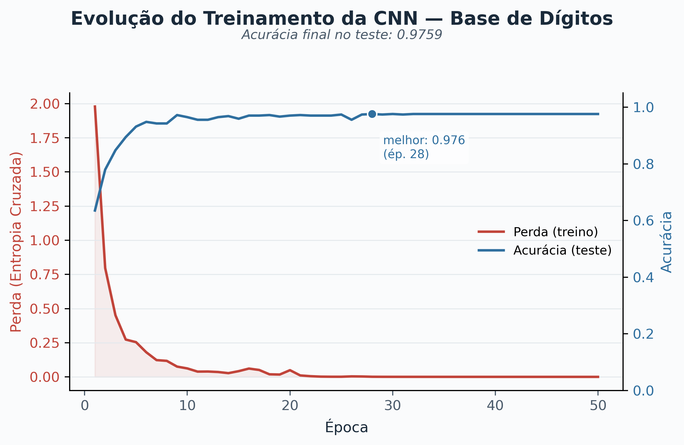
The learning curves resulting from this process are shown in Figure 9.15, generated at the end of execution.

1. Training Phase (modelo_cnn.train()): The main loop executes training over \(50\) epochs. In each epoch, the following steps occur:

   • Stochastic Shuffling: The function torch.randperm(n) generates a random permutation of the sample indices, ensuring that the ordering of mini-batches varies each epoch to avoid sampling biases.
   • Division into Mini-batches: The training set is sliced into batches of \(32\) samples (tam_lote = 32).
   • Zeroing Gradients (otimizador.zero_grad()): Clears the gradients accumulated in the tensor from the previous iteration, preventing the unwanted summation of derivatives across distinct batches.
   • Forward Pass and Loss: The forward pass computes the predictions saida, and the call criterio(saida, y_treino_t[idx]) quantifies the batch error.
   • Backpropagation (perda.backward()): Applies the chain rule to compute the partial derivatives of the loss with respect to each parameter (\(\frac{\partial L}{\partial w}\)).
   • Weight Update (otimizador.step()): Updates the model parameters according to the Adam optimizer equations.

2. Evaluation Phase (modelo_cnn.eval()): At the end of each epoch, the model is switched to evaluation mode. The context with torch.no_grad() temporarily disables the automatic derivative computation engine (autograd), reducing memory consumption and accelerating inference on the test set (X_teste_t). The operation .argmax(dim=1) extracts the class with the highest probability for each sample, allowing the test accuracy to be calculated.

3. Visualization with the morph Library: The function mm.showTrainCurves from the didactic library morph consolidates the training loss history and test accuracy into a single graphical panel, allowing the model convergence to be diagnosed and the stability of learning to be monitored across epochs.

# 4. Training Loop (Mini-batch SGD)
n = X_treino_t.size(0)                    # Number of samples
tam_lote = 32                             # Mini-batch size
epocas = 50                               # Total epochs
historico_perda, historico_acc = [], []   # Metrics history

for epoca in range(epocas):                  # Repeat for each epoch
    modelo_cnn.train()                       # Training mode
    perm = torch.randperm(n)                 # Shuffle samples
    perda_epoca = 0.0                        # Accumulate losses
    for i in range(0, n, tam_lote):          # Iterate over mini-batches
        idx = perm[i:i + tam_lote]           # Batch indices
        otimizador.zero_grad()               # Zero gradients
        saida = modelo_cnn(X_treino_t[idx])  # Forward pass
        perda = criterio(saida, y_treino_t[idx]) # Compute loss
        perda.backward()                         # Backpropagation
        otimizador.step()                        # Update weights
        perda_epoca += perda.item() * len(idx)   # Sum loss

    # Model evaluation on the test set at the end of each epoch
    modelo_cnn.eval()                            # Evaluation mode
    with torch.no_grad():                        # No gradients
        pred_teste = modelo_cnn(X_teste_t).argmax(dim=1)  # Predictions
        acc_teste = (pred_teste == y_teste_t).float().mean().item()  # Accuracy
    historico_perda.append(perda_epoca / n)      # Record loss
    historico_acc.append(acc_teste)              # Record accuracy

acc_final_cnn = historico_acc[-1]                # Final accuracy
print(f"Final accuracy of the CNN on the test set: {acc_final_cnn:.4f}")  # Display result

final = mm.showTrainCurves(                      # Plot curves
    historico_perda, historico_acc,
    titulo="Evolução do Treinamento da CNN — Base de Dígitos",
    subtitulo=f"Acurácia final no teste: {acc_final_cnn:.4f}",
)

Final accuracy of the CNN on the test set: 0.9759

Figure 9.15: Training and evaluation curves of the CNN on the digits dataset: evolution of cross-entropy loss on the training set and accuracy on the test set over 50 epochs.

9.5.1.1.5 Block 5: Visualization of the Activation Flow

Inspecting the trained network allows observing the progressive transformation of the input tensor across the layers of the CNNDigitos architecture. Figure 9.16 illustrates the dimensions and intermediate activations obtained when processing a real example of the digit \(3\).

1. Sample Selection and Preparation: The stochastic seed is fixed with torch.manual_seed(7) to ensure reproducibility of the results. The first occurrence of the digit \(3\) in the load_digits dataset is isolated, normalized to the interval \([0.0, 1.0]\), and reshaped as a tensor x of dimension \((1, 1, 8, 8)\).

2. Intermediate Inspection with mm.showNet: The mm.showNet function from the morph library performs the forward pass of the tensor x through the previously trained modelo_cnn instance. Using forward hooks, the function intercepts the numerical state of activations in the convolutional (nn.Conv2d), pooling (nn.MaxPool2d), and fully connected (nn.Linear) layers, returning them in the acts dictionary. The nonlinear activation functions (nn.ReLU) are not registered as independent stages, since their application occurs directly on the output tensor of the corresponding layer.

3. Result Verification: The command list(acts.keys()) displays the sequence of identifiers for the monitored layers, allowing confirmation of the progressive dimensional reduction and the generation of the logit with maximum value at the index corresponding to class \(3\), as demonstrated in Figure 9.16.

torch.manual_seed(7)
digits = load_digits()
idx = np.where(digits.target == 3)[0][0]
img = digits.images[idx] / 16.0
x = torch.tensor(img, dtype=torch.float32).view(1, 1, 8, 8)

# Reuse of the previously trained model instance
acts = mm.showNet(
    modelo_cnn,
    x,
    titulo="Fluxo de transformações dos tensors ao longo da arquitetura CNNDigitos",
    subtitulo=f"Exemplo real do dataset load_digits (classe verdadeira: {digits.target[idx]})",
)
print("Captured layers:", list(acts.keys()))

Figure 9.16: Flow of activations of the trained CNN when processing a real example of the digit 3, from the load_digits dataset: tensor dimensions layer by layer, from input to output logit.

Captured layers: ['conv1', 'pool', 'conv2', 'pool #2', 'fc1', 'fc2']

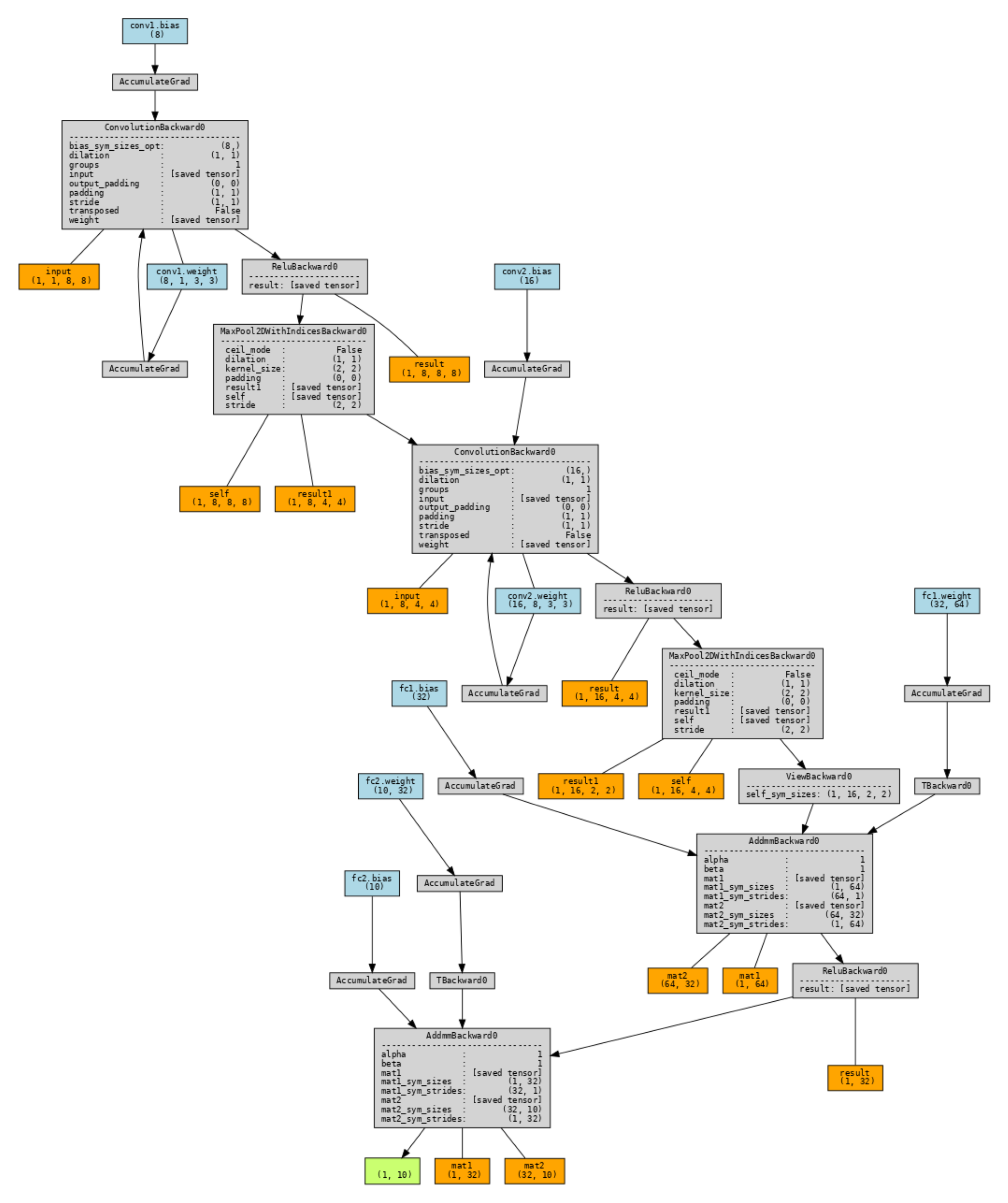
9.5.1.1.6 Inspecting the Computational Graph with torchviz

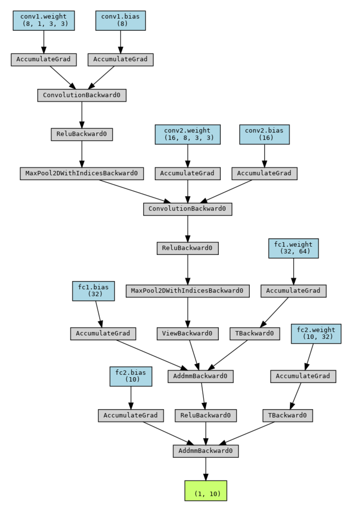
While mm.showNet prioritizes didactic clarity—displaying one column per layer with trainable parameters—the torchviz library projects the autograd graph exactly as PyTorch builds it internally for gradient computation. Figure 9.17 illustrates this perspective by representing the CNNDigitos architecture.

1. Tracked Forward Propagation: With the trained model in eval() mode, the forward pass over the x tensor of digit \(3\) is sufficient for the autograd engine to record all executed operations, including those without trainable parameters, such as the ReLU activation function and the view dimensional reshaping.

2. Graph Generation (make_dot): The make_dot(saida, params=...) function builds the graph from the output tensor by traversing backward through the operation history to the leaf nodes (the model’s trainable parameters). Each node in the diagram represents an operation of the backward pass (such as ReluBackward or AddmmBackward), not merely a conceptual block of the nn.Module.

3. Export and Rendering (.render): The .render(..., format="png", cleanup=True) method invokes the dot executable from Graphviz to compile the image in PNG format, automatically removing intermediate source-code files.

Figure 9.17 highlights how this computational graph, even for a compact architecture, exhibits greater density than the mm.showNet panel, as it details each atomic operation responsible for the gradient flow.

# 1. Forward pass with gradient tracking enabled
modelo_cnn.eval()
saida = modelo_cnn(x)  # Reuse of tensor x (digit 3)

# 2. Basic graph: flow of operations up to the output
grafo_simples = make_dot(saida, params=dict(modelo_cnn.named_parameters()))
caminho_simples = grafo_simples.render("cnn_digitos_grafo_simples", format="png", cleanup=True)

# 3. Direct display in the Quarto/Jupyter environment
# The .render() returns the path of the generated PNG file; we need to open it as an image
imagem_simples = np.array(Image.open(caminho_simples).convert("RGB"))
mm.show(imagem_simples, figsize=(5,10))

Figure 9.17: Computational graph of CNNDigitos generated via torchviz, showing the forward operations and the gradient nodes (backward) associated with each trainable parameter.

9.5.1.1.7 Detailed View of the Computational Graph with torchviz

In addition to the simplified representation, the torchviz library allows expanding the autograd graph to inspect the internal execution details of the CNNDigitos network. Figure 9.18 presents this expanded structure for the same input tensor x.

1. Tracing with Operation Attributes (show_attrs=True): The inclusion of attributes displays the hyperparameter configurations associated with each computational node during the forward pass, such as kernel dimensions (kernel_size), strides, and paddings in convolutions and subsamplings.

2. Detection of Saved Tensors in Memory (show_saved=True): This parameter forces the explicit display of the intermediate tensors that PyTorch retains in memory during the forward pass. These data are preserved because they will be strictly necessary for calculating the partial derivatives during the backward pass.

3. Generation and Compilation of Graphs: While grafo_simples generates a direct view of the gradient flow, grafo_detalhado compiles the expanded graph into the file cnn_digitos_grafo_detalhado.png via the dot executable from Graphviz.

As observed in Figure 9.18, this detailed visualization is useful for debugging video memory (VRAM) consumption and verifying how the PyTorch engine internally allocates each node of the chain rule.

# same code as before (make_dot + render)...

# 2. Detailed graph: display of dimensions and tensors saved for backward
grafo_detalhado = make_dot(
    saida,
    params=dict(modelo_cnn.named_parameters()),
    show_attrs=True,   # Displays operation attributes (e.g., kernel_size, stride)
    show_saved=True,   # Displays tensors saved in memory for backpropagation
)

caminho_detalhado = grafo_detalhado.render("cnn_digitos_grafo_detalhado", 
                                           format="png", cleanup=True)

# 3. Direct display in the Quarto/Jupyter environment
imagem_detalhado = np.array(Image.open(caminho_detalhado).convert("RGB"))
mm.show(imagem_detalhado, figsize=(8, 16))

Figure 9.18: Detailed graph of the CNNDigitos class generated via torchviz.

9.5.1.1.8 Comparison with Chapter 7

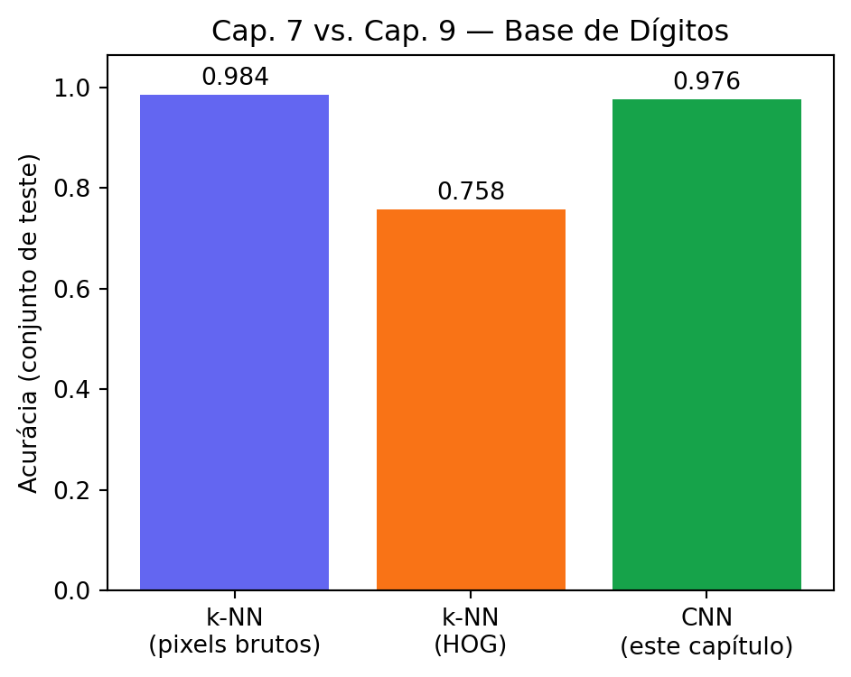
Figure 9.19 brings together the results obtained on the same dataset (load_digits), establishing a direct parallel between the classical approaches explored previously and the CNN developed in this chapter.

1. Performance of Raw Pixels vs. Manual Descriptors: In the experiments from Chapter 7, the \(k\text{-NN}\) classifier (\(k=3\)) achieved an accuracy of \(98.4\%\) when fed directly with the raw pixels of the images. In contrast, prior feature extraction via the Histogram of Oriented Gradients (HOG) resulted in significantly lower performance (\(75.8\%\)). This decline occurs because HOG was designed to capture edge gradients in higher-resolution images; in matrices of only \(8 \times 8\) pixels, the spatial resolution is insufficient to form informative orientation histograms.

2. Equivalence of CNN and End-to-End Learning: The convolutional network CNNDigitos achieves competitive performance of \(97.6\%\), approaching the accuracy of \(k\text{-NN}\) with raw pixels on a small and pre-aligned dataset. The major conceptual advantage lies in representation learning: instead of relying on manually designed descriptors (handcrafted features) or keeping the entire dataset in memory for neighbor searching at inference time, the CNN automatically optimizes its own convolutional filters during training, yielding a compact model capable of performing feature extraction and classification in an integrated (end-to-end) manner.

import matplotlib.pyplot as plt

# Values obtained in Chapter 7 (k-NN, k=3), reproduced for direct comparison
ACC_KNN_PIXELS_CAP7 = 0.9844
ACC_KNN_HOG_CAP7 = 0.7578

metodos = ["k-NN\n(pixels brutos)", "k-NN\n(HOG)", "CNN\n(este capítulo)"]
acuracias = [ACC_KNN_PIXELS_CAP7, ACC_KNN_HOG_CAP7, acc_final_cnn]

plt.figure(figsize=(5, 4))
cores = ["#6366f1", "#f97316", "#16a34a"]
plt.bar(metodos, acuracias, color=cores)
plt.ylim(0, max(acuracias) + 0.08)
plt.ylabel("Acurácia (conjunto de teste)")
plt.title("Cap. 7 vs. Cap. 9 — Base de Dígitos")

for i, v in enumerate(acuracias):
    plt.text(i, v + 0.02, f"{v:.3f}", ha="center")

plt.tight_layout()
plt.show()

Figure 9.19: Comparison of accuracy between the classic classifiers from Chapter 7 (raw pixels and HOG with k-NN) and the CNN trained in this chapter, on the same digit dataset.

Note🧠 Why It Works — And Why the CNN Does Not Always “Win”

The observed result here repeats the pattern already seen in Chapter 7: the CNN, despite automatically learning its features, does not necessarily outperform the \(k\text{-NN}\) with raw pixels on this specific dataset. The explanation is the same: load_digits is a small dataset (fewer than \(1,800\) examples), with images that are already centered, normalized, and of very low resolution (\(8 \times 8\)) — conditions under which direct comparison of intensities is already highly informative, and there is little data for the network to learn filters that are truly superior to simple descriptors.

The real differentiator of CNNs appears in scenarios that handcrafted descriptors and simple classifiers cannot address: larger and more realistic images, with thousands of categories, substantial variation in pose, lighting, and background, and massive training sets — exactly the regime in which the models presented in the section “Large-Scale Applications”, later on, were trained. The pedagogical lesson that runs through Chapters 7, 8, and 9 of this book is consistent: the sophistication of a method should be proportional to the complexity of the problem — using a CNN for a problem that a \(k\text{-NN}\) solves equally well is a waste of computational resources, not a virtue.

This same proportionality applies to the inspection tools used throughout the chapter. The mm.showNet was built for didactic purposes and works well on shallow networks such as CNNDigitos, but it does not scale to deep architectures: each traced layer becomes a column in the figure, and convolutional layers with hundreds of channels generate mosaics too large for visual interpretation; furthermore, the hooks store all activations in memory, and the layout assumes a sequential flow, not faithfully representing residual connections or branches (as in ResNets or Inception modules). Thus, showNet should be understood as a pedagogical lens for small networks — analogous to the role of mm.showBoundBox in the visual debugging of detections — and not as a substitute for production-oriented tools such as TensorBoard or torchviz.

9.5.1.2 Transfer Learning

Training a CNN from scratch generally requires a large amount of labeled data and significant computational resources, as the training process must adjust all network parameters. In many applications, however, only a reduced set of data is available for the task of interest. In this situation, transfer learning reuses the representations learned by a model previously trained on a source task with a large volume of data, reducing training costs and the need for new samples.

In CV, this strategy explores the hierarchical organization of CNNs. The initial layers learn low-level visual features, such as edges, textures, intensity gradients, and color patterns, which remain useful across different domains. The deeper layers combine this information to form progressively more abstract and specialized representations, related to the classes present in the training base.

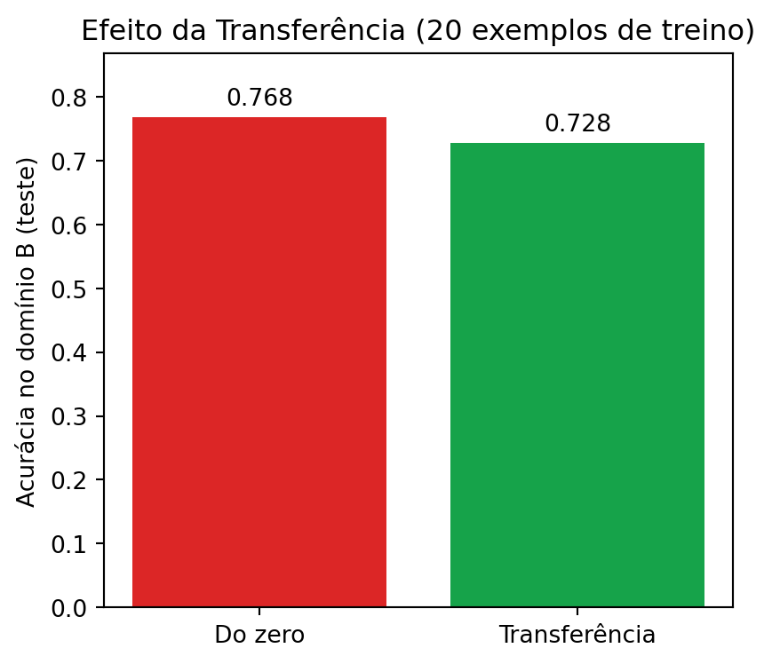
This section investigates under what conditions transfer learning yields good results. The first experiment shows that a small extractor trained on a restricted domain can lead to negative transfer. The second demonstrates why deep models pre-trained on large image datasets achieve high performance on new tasks. Finally, the third applies this strategy to a plant health diagnosis problem, illustrating a scenario close to real-world applications.

9.5.1.2.1 Experiment 1 — Limitations of a Small and Specialized Extractor

The first experiment shows that transfer learning does not always improve a model’s performance. To this end, the handwritten digits dataset (load_digits) is divided into two disjoint domains:

• Domain A (source): digits \(0\) to \(4\), used to train a small CNN;
• Domain B (target): digits \(5\) to \(9\), reindexed to \(0\) to \(4\), forming a new task with only \(20\) training samples.

The objective is to evaluate the effect of reusing the feature extractor learned in Domain A without allowing its adaptation to Domain B.

9.5.1.2.1.1 Block 1: Division of Domains, Scarcity, and Display of Samples

This block prepares the dataset for the experiment. Unlike the previous project, which used all digits in a single classification problem, the dataset is divided into two independent tasks: a source task (Domain A) and a target task (Domain B).

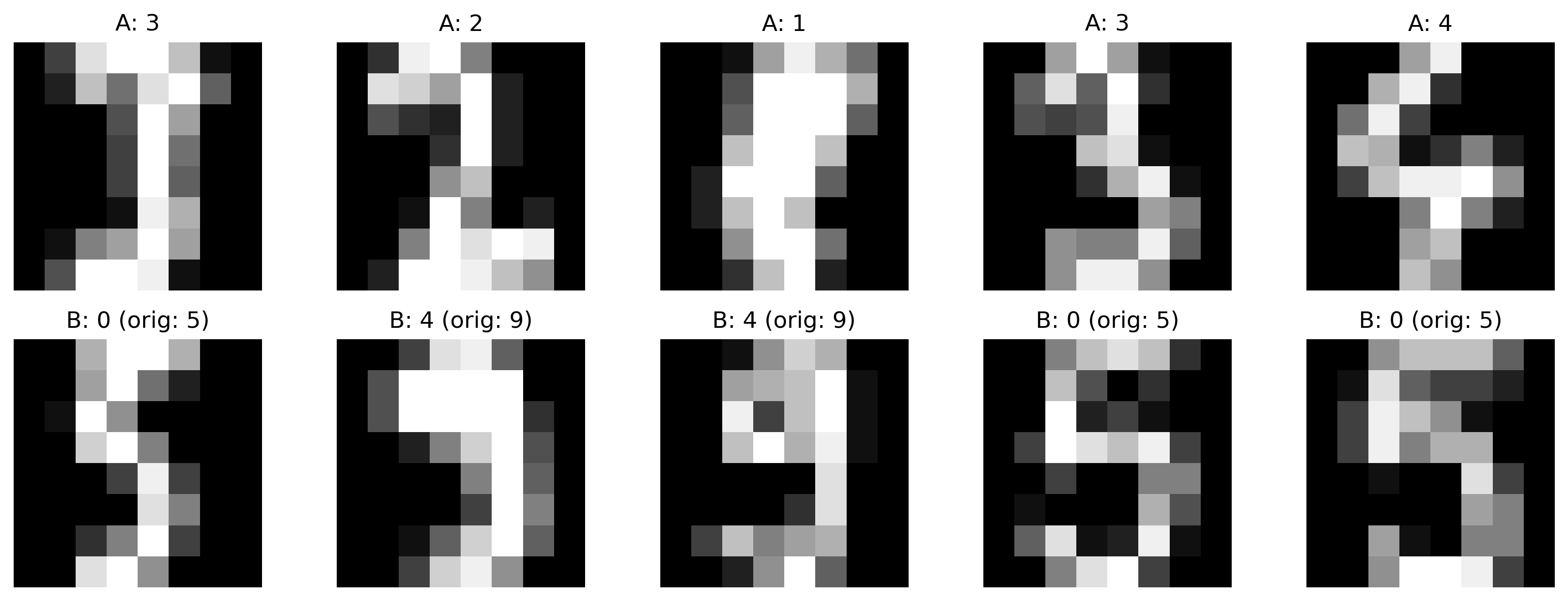
Figure 9.20 presents examples from both domains after class separation, conversion to PyTorch tensors, and preprocessing.

1. Class separation: The boolean masks mask_A and mask_B separate the examples from each domain. Next, the code reindexes the labels of Domain B (y[mask_B] - 5) to the range \([0,4]\), allowing both models to use five output classes.

2. Data scarcity: The generator np.random.default_rng(0) selects only \(20\) samples for training Domain B, approximately four per class, simulating a scenario where training from scratch tends to suffer from overfitting.

3. Conversion to tensors: The para_tensor function converts the images to the format \((N,1,8,8)\) and the labels to torch.long, compatible with the nn.Conv2d layers and the loss function.

4. Sample visualization: The code uses .squeeze().numpy() to convert the tensors into NumPy arrays. Figure 9.20 presents examples from both domains and highlights the reindexing applied to the labels of Domain B.

# 1. Splitting the dataset into two disjoint domains
classes_A, classes_B = [0, 1, 2, 3, 4], [5, 6, 7, 8, 9]
mask_A, mask_B = np.isin(y, classes_A), np.isin(y, classes_B)

XA, yA = X[mask_A], y[mask_A]
XB, yB = X[mask_B], y[mask_B] - 5  # Reindexing the labels to the range [0, 4]

# Splitting into training and test sets for both domains
XA_tr, XA_te, yA_tr, yA_te = train_test_split(
    XA, yA, test_size=0.25, random_state=42, stratify=yA
)
XB_tr, XB_te, yB_tr, yB_te = train_test_split(
    XB, yB, test_size=0.25, random_state=42, stratify=yB
)

# Simulation of extreme scarcity in the target domain: only 20 training samples
rng = np.random.default_rng(0)
idx_poucos = rng.choice(len(XB_tr), size=20, replace=False)
XB_tr_poucos, yB_tr_poucos = XB_tr[idx_poucos], yB_tr[idx_poucos]

# Helper function for conversion into PyTorch tensors
def para_tensor(Ximg, yarr):
    return torch.tensor(Ximg).unsqueeze(1), torch.tensor(yarr, dtype=torch.long)

XA_tr_t, yA_tr_t = para_tensor(XA_tr, yA_tr)
XA_te_t, yA_te_t = para_tensor(XA_te, yA_te)
XB_tr_t, yB_tr_t = para_tensor(XB_tr_poucos, yB_tr_poucos)
XB_te_t, yB_te_t = para_tensor(XB_te, yB_te)

# Display of samples from both domains
n_amostras = 5
imgs_A = [img.squeeze().numpy() for img in XA_tr_t[:n_amostras]]
titles_A = [f"A: {label.item()}" for label in yA_tr_t[:n_amostras]]

imgs_B = [img.squeeze().numpy() for img in XB_tr_t[:n_amostras]]
titles_B = [f"B: {label.item()} (orig: {label.item()+5})" for label in yB_tr_t[:n_amostras]]

mm.show(
    imgs_A + imgs_B,
    titles=titles_A + titles_B,
    cols=n_amostras,
    figsize=(12, 4.5)
)

Figure 9.20: Samples from the training sets after preprocessing and dimensionality adjustment to PyTorch tensors: Domain A (digits 0 to 4, source task) and Domain B (digits 5 to 9 reindexed to 0 to 4, target task).

9.5.1.2.1.2 Block 2: Modular Architecture and Generic Routines

To enable learning transfer, the convolutional architecture and training loop were refactored relative to the CNNDigitos class from the previous project.

1. Architecture Modularization (Difference from CNNDigitos):

   • In the previous project, the CNNDigitos class declared all layers (conv1, conv2, pool, fc1, fc2) as direct members of a single monolithic class.
   • Here, the architecture is separated into two components: the ExtratorConv class encapsulates the convolutional spatial block (\(2\) \(3 \times 3\) convolutions, \(2\) \(2 \times 2\) Max-Poolings, and flattening to \(64\) elements), while the CNNCompleta class instantiates this extractor in self.extrator and attaches the classifier “head” (fc1 and fc2).
   • This separation is what allows the internal state of the extractor (state_dict()) to be copied from one model to another in an isolated manner.

2. Adjustment in the Number of Output Classes: While CNNDigitos in the previous project had \(10\) logits in the output layer (self.fc2 = nn.Linear(32, 10)), the CNNCompleta class receives n_classes=5 in the constructor to suit the division of domains \(A\) and \(B\).

3. Flexibilization of the Training Loop (treinar):

   • In the previous project, the training loop iterated directly over the model’s global attributes (modelo_cnn.parameters()) and computed specific metrics inline.
   • The treinar function abstracts this process and introduces the optional parameter parametros. If provided, the Adam optimizer updates only the parameters in that list, ignoring layers whose gradients have been deactivated. This flexibility is crucial for performing training with partial freezing of the network.

4. Isolation of Evaluation (calcular_acuracia): As done in the testing phase of the previous project, the function sets the model to eval() and uses the torch.no_grad() context to deactivate autograd, computing accuracy via .argmax(dim=1).

# Definition of the reusable convolutional block (same extraction as the previous project)
class ExtratorConv(nn.Module):
    def __init__(self):
        super().__init__()
        self.conv1 = nn.Conv2d(1, 8, 3, padding=1)
        self.conv2 = nn.Conv2d(8, 16, 3, padding=1)
        self.pool = nn.MaxPool2d(2, 2)
        self.relu = nn.ReLU()

    def forward(self, x):
        x = self.pool(self.relu(self.conv1(x)))
        x = self.pool(self.relu(self.conv2(x)))
        return x.view(x.size(0), -1)

# Modular architecture combining the extractor and the classification head
class CNNCompleta(nn.Module):
    def __init__(self, n_classes=5):
        super().__init__()
        self.extrator = ExtratorConv()
        self.fc1 = nn.Linear(64, 32)
        self.fc2 = nn.Linear(32, n_classes)
        self.relu = nn.ReLU()

    def forward(self, x):
        x = self.extrator(x)
        x = self.relu(self.fc1(x))
        return self.fc2(x)

# Generic training routine with selective parameter optimization
def treinar(modelo, X_t, y_t, epocas, lr, tam_lote=16, parametros=None):
    # Trainable parameters
    params = parametros if parametros is not None else modelo.parameters()  
    otim = optim.Adam(params, lr=lr)               # Adam optimizer
    crit = nn.CrossEntropyLoss()                   # Loss function
    n_amostras = X_t.size(0)                       # Number of samples
    for _ in range(epocas):                        # Repeat per epoch
        perm = torch.randperm(n_amostras)          # Shuffles samples
        for i in range(0, n_amostras, tam_lote):   # Iterates over mini-batches
            idx = perm[i:i + tam_lote]             # Batch indices
            otim.zero_grad()                       # Zeros gradients
            perda = crit(modelo(X_t[idx]), y_t[idx])  # Computes loss
            perda.backward()                       # Backpropagation
            otim.step()                            # Updates weights

# Evaluation routine
def calcular_acuracia(modelo, X_t, y_t):
    modelo.eval()                                  # Evaluation mode
    with torch.no_grad():                          # No gradients
        pred = modelo(X_t).argmax(dim=1)           # Predicted classes
    return (pred == y_t).float().mean().item()     # Returns accuracy

9.5.1.2.1.3 Block 3: Pre-training, Transfer, and Comparative Analysis

This block carries out a comparison between training the model from scratch and applying transfer learning with static freezing of the feature extractor. To ensure full transparency of the experiment, the sizes of the training and test sets for both domains are printed to the terminal.

1. Quantification of Samples per Domain:

   • Domain A (source, digits \(0\) to \(4\)): It comprises \(675\) training samples (\(75\%\)) and \(226\) test samples (\(25\%\)), providing abundant data for the source_model to learn the convolutional feature extractor until it reaches \(100\%\) accuracy.
   • Domain B (target, digits \(5\) to \(9\)): It has \(224\) test samples in total, but its training set is intentionally reduced from \(672\) to only \(20\) samples (XB_tr_few), creating a severe scenario of data scarcity.

2. Step 1: Pre-training on Domain A (Source): The source_model is trained from scratch on the \(675\) samples of digits \(0\) to \(4\). Over \(40\) epochs, the convolutional feature extractor adjusts its filters to identify the distinctive features of these first five digits, reaching \(100\%\) accuracy on the test set (\(226\) samples).

3. Step 2: Weight Transfer and Freezing:

   • The transfer_model is created to solve the Domain B task (digits \(5\) to \(9\)).

   • The weights learned on Domain A are copied via:

     • load_state_dict(source_model.extractor.state_dict())

   • Freezing: The loop for p in transfer_model.extractor.parameters(): p.requires_grad = False disables gradient computation in the convolutional layers.

   • Selective Training: The train(...) call strictly passes the parameters of the dense layers (head_params), adjusting the classification head with only the \(20\) training samples.

4. Step 3: Training from Scratch on Domain B (Experimental Control): The from_scratch_model has the same architecture but is trained from scratch on the same \(20\) samples from Domain B, without any weight reuse, over the same \(40\) epochs.

5. Analysis of Results (Figure 9.21):

   • With Frozen Transfer (\(72.77\%\)): By reusing the feature extractor trained on Domain A and freezing its parameters, the network achieves \(72.77\%\) test accuracy (\(224\) samples) by adjusting only the dense layers.
   • Trained from Scratch (\(76.79\%\)): Training from scratch outperforms frozen transfer on the Domain B test set.
   • Reason for the Difference: Since it is a tiny model (only \(16\) convolutional filters on \(8 \times 8\) matrices), the feature extractor trained on Domain A became hyperspecialized in the geometric shapes of digits \(0\) to \(4\). By rigidly freezing these few filters, the target model was limited to detectors unsuitable for \(5\) to \(9\). The network trained from scratch, even with only \(20\) samples, was able to adapt its \(16\) filters directly to the features of Domain B.

# Fix seed for reproducibility
torch.manual_seed(42)

# Display training and test group sizes
print("=== Database Size Breakdown ===")
print(f"Domain A (0-4) — Training: {len(XA_tr_t)} samples | Test: {len(XA_te_t)} samples")
print(f"Domain B (5-9) — Full training: {len(XB_tr)} | Reduced training: {len(XB_tr_poucos)}",
      f"| Test: {len(XB_te_t)} samples\n")

# 1. Pre-training on the source task (Domain A: digits 0-4)
modelo_origem = CNNCompleta(n_classes=5)                       # Create CNN

#######
treinar(modelo_origem, XA_tr_t, yA_tr_t, epocas=40, lr=1e-2)   # Train model
         
acc_A = calcular_acuracia(modelo_origem, XA_te_t, yA_te_t)     # Measure accuracy
                          
print(f"Accuracy in source domain A "                      # Display result
      f"(digits 0-4, {len(XA_te_t)} tests): " f"{acc_A:.4f}"# Display result
      f"(dígitos 0-4, {len(XA_te_t)} testes): " f"{acc_A:.4f}")

# 2. Transfer Learning (Frozen Extractor)
modelo_transferencia = CNNCompleta(n_classes=5)        # Create CNN
modelo_transferencia.extrator.load_state_dict(         # Copy extractor
    modelo_origem.extrator.state_dict())

for p in modelo_transferencia.extrator.parameters():   # Traverse extractor
    p.requires_grad = False                            # Freeze weights

params_cabeca = list(modelo_transferencia.fc1.parameters())  # FC1
params_cabeca += list(modelo_transferencia.fc2.parameters()) # +FC2

#######
treinar(modelo_transferencia, XB_tr_t, yB_tr_t,              # Train head
         epocas=40, lr=1e-2, parametros=params_cabeca)

acc_transferencia = calcular_acuracia(modelo_transferencia, XB_te_t, yB_te_t) # Measure accuracy

# 3. Training from Scratch in Domain B
modelo_do_zero = CNNCompleta(n_classes=5)                     # Create CNN

#######
treinar(modelo_do_zero, XB_tr_t, yB_tr_t, epocas=40, lr=1e-2) # Train model
         
acc_do_zero = calcular_acuracia(modelo_do_zero,  XB_te_t, yB_te_t) # Measure accuracy
                               

print(f"Target domain B (digits 5-9), only {len(XB_tr_poucos)} ", 
      f"training examples ({len(XB_te_t)} tests):")
print(f"  With transfer (frozen extractor): {acc_transferencia:.4f}")
print(f"  Training from scratch (same data/epochs): {acc_do_zero:.4f}")

# Comparative visualization
plt.figure(figsize=(4.5, 4))
plt.bar(["Do zero", "Transferência"], [acc_do_zero, acc_transferencia], 
        color=["#dc2626", "#16a34a"])
plt.ylim(0, max([acc_do_zero, acc_transferencia]) + 0.1)
plt.ylabel("Acurácia no domínio B (teste)")
plt.title(f"Efeito da Transferência ({len(XB_tr_poucos)} exemplos de treino)")

for i, v in enumerate([acc_do_zero, acc_transferencia]):
    plt.text(i, v + 0.02, f"{v:.3f}", ha="center")

plt.tight_layout()
plt.show()

=== Database Size Breakdown ===
Domain A (0-4) — Training: 675 samples | Test: 226 samples
Domain B (5-9) — Full training: 672 | Reduced training: 20 | Test: 224 samples

Accuracy in source domain A (digits 0-4, 226 tests): 1.0000(dígitos 0-4, 226 testes): 1.0000
Target domain B (digits 5-9), only 20  training examples (224 tests):
  With transfer (frozen extractor): 0.7277
  Training from scratch (same data/epochs): 0.7679

Figure 9.21: Comparison of accuracy on the Domínio B test set (digits 5 to 9) under data restriction (20 training examples): demonstration of the impact of rigid freezing and negative transfer in low-capacity networks.

9.5.1.2.1.4 Block 4: Visualization of the Activation Flow with mm.showNet

To confirm that the reused feature extraction preserves the dimensional transformations studied in the previous project, the mm.showNet function from the morph library is used again. Figure 9.22 displays the activation flow of modelo_transferencia when processing a sample from Domain B (digit \(7\), reindexed to class \(2\)).

1. Preservation of the Convolutional Flow: Since the ExtratorConv architecture replicates the same convolution and pooling layers as the CNNDigitos from the previous project, the dimensions of the intermediate tensors remain at \((1, 8, 4, 4)\) in the first block.
2. Inspection of the Adapted Head: The difference from the previous project arises in the output layer (fc2): whereas the previous project’s model projected the intermediate vector into \(10\) logits (classes \(0\) through \(9\)), the transfer model projects the vector into \(5\) logits (classes \(0\) through \(4\)), capturing the relative probabilities of Domain B.

# Selects the first test sample from Domain B
x_amostra_B = XB_te_t[0:1]  # Tensor of dimension (1, 1, 8, 8)
classe_verdadeira = yB_te_t[0].item()
classe_original = classe_verdadeira + 5

# Inspection of the activation flow in the transfer model
acts_transfer = mm.showNet(
    modelo_transferencia,
    x_amostra_B,
    titulo="Fluxo de ativações no modelo de transferência (Domínio B)",
    subtitulo=f"Amostra do dígito {classe_original} (rótulo reindexado: {classe_verdadeira})",
)

print("Layers captured in the transfer model:\n", list(acts_transfer.keys()))

Figure 9.22: Flow of activations and dimensional transformations of the tensors in the transfer learning model when processing a test sample from Domain B (digit 7, reindexed to class 2).

Layers captured in the transfer model:
 ['extrator.conv1', 'extrator.pool', 'extrator.conv2', 'extrator.pool #2', 'fc1', 'fc2']

9.5.1.2.1.5 Analysis of Experiment 1

The model trained from scratch achieves superior accuracy compared to the model with transfer learning and a frozen feature extractor. This result characterizes a case of negative transfer and stems from three factors:

1. Low capacity: The feature extractor has only \(16\) filters of size \(3 \times 3\), insufficient to learn generalizable representations.

2. Domain specialization: Training on digits \(0\) through \(4\) produces filters that are poorly discriminative for digits \(5\) through \(9\).

3. Lack of adaptation: Freezing prevents the feature extractor from adjusting its filters to the new task.

Note💡 Pedagogical Prompt

This experiment uses a small feature extractor trained on a restricted domain. Would the result be different if the feature extractor had learned its representations on a dataset with millions of images and great object diversity?

9.5.1.2.2 Experiment 2 — When Transfer Actually Works (Pre-trained ResNet-18)

The second experiment repeats the same structure as the first — few training examples, two classes, comparison between strategies — but replaces the handcrafted extractor of \(16\) filters with the ResNet-18, an \(18\)-layer architecture pre-trained on ImageNet (\(1.4\) million images, \(1,000\) categories), and the synthetic digit dataset with real photographs from the Oxford-IIIT Pet Dataset (PARKHI, 2012).

The task: distinguish two canine breeds — Pug and Boxer — from only \(15\) training photographs per class.

Tip🐶 Why this scenario?

The challenge here is not the visual similarity between the breeds — Pug and Boxer have quite distinct sizes and proportions — but rather the scarcity of data: only \(30\) real photographs in total, with no synthetic images whatsoever. It is the type of low-data-budget problem that, in practice, motivates the use of pre-trained networks: there is neither time nor resources to photograph and label thousands of dogs before training a classifier from scratch.

9.5.1.2.2.1 Block 1: Loading the Real Dataset and Sparse Sampling

1. Source: the Oxford-IIIT Pet Dataset (PARKHI, 2012) is loaded via torchvision.datasets.OxfordIIITPet, which automatically downloads the \(7,349\) photographs and their breed labels on the first run.
2. Filtering: only the two breeds of interest (Pug, Boxer) are kept.
3. Deliberate sparsity: only \(15\) training photographs per class (\(30\) in total) are sampled — the remainder constitutes the test set, used exclusively for evaluation.

Figure 9.23 displays training samples for each breed.

import random

RACAS_ALVO = ["Pug", "Boxer"]
N_TREINO_POR_CLASSE = 15
N_TESTE_POR_CLASSE = 20

# 1. Download of the full dataset (37 breeds) — CC BY-SA 4.0 license
pets_completo = OxfordIIITPet(
    root="dados_pets", split="trainval", target_types="category", download=True
)
nomes_racas = pets_completo.classes
indices_alvo = [nomes_racas.index(r) for r in RACAS_ALVO]

# 2. Filtering of the two breeds of interest, separated by class
por_classe = {idx: [] for idx in indices_alvo}
for img, lbl in pets_completo:
    if lbl in indices_alvo:
        por_classe[lbl].append(img)

# 3. Sampling: few training images, more test images
rng = random.Random(42)
imgs_treino, y_treino, imgs_teste, y_teste = [], [], [], []
for classe_idx, idx_original in enumerate(indices_alvo):
    imgs_raca = por_classe[idx_original][:]
    rng.shuffle(imgs_raca)
    imgs_treino += imgs_raca[:N_TREINO_POR_CLASSE]
    y_treino += [classe_idx] * N_TREINO_POR_CLASSE
    imgs_teste += imgs_raca[N_TREINO_POR_CLASSE : N_TREINO_POR_CLASSE + N_TESTE_POR_CLASSE]
    y_teste += [classe_idx] * N_TESTE_POR_CLASSE

print(f"Training: {len(imgs_treino)} images | Test: {len(imgs_teste)} images")

amostras_pil = imgs_treino[:4] + imgs_treino[N_TREINO_POR_CLASSE:N_TREINO_POR_CLASSE + 4]
amostras_exibicao = [np.array(img.convert("RGB")) for img in amostras_pil]  # PIL -> ndarray
titulos_exibicao = [RACAS_ALVO[0]] * 4 + [RACAS_ALVO[1]] * 4
mm.show(amostras_exibicao, titles=titulos_exibicao, cols=4, figsize=(11, 6))

Figure 9.23

9.5.1.2.2.2 Block 2: Three Strategies on the Same Architecture

To isolate the effect of transfer learning, the three strategies reuse exactly the same architecture (ResNet-18), differing only in the origin of the weights and which parameters remain trainable:

1. from_scratch: random weights (weights=None) — equivalent to training the ResNet-18 architecture entirely from scratch, as in Block 2 of Experiment 1.
2. frozen: weights pre-trained on ImageNet, with requires_grad = False in all convolutional layers — only the new final layer is trained.
3. fine_tuning: weights pre-trained on ImageNet as a starting point, but without freezing — the entire network adapts to the new domain, with a low learning rate to avoid destroying prior knowledge.

In all cases, the final layer fc is replaced by nn.Linear(fc.in_features, 2), corresponding to the two target breeds.

transformacao_resnet = T.Compose([
    T.Resize((224, 224)),
    T.ToTensor(),
    T.Normalize(mean=[0.485, 0.456, 0.406], std=[0.229, 0.224, 0.225]),
])

def prepara_tensores(imgs, labels):
    X = torch.stack([transformacao_resnet(img.convert("RGB")) for img in imgs])
    y = torch.tensor(labels, dtype=torch.long)
    return X, y

X_tr, y_tr = prepara_tensores(imgs_treino, y_treino)
X_te, y_te = prepara_tensores(imgs_teste, y_teste)

def cria_modelo_pets(estrategia):
    pesos = None if estrategia == "do_zero" else models.ResNet18_Weights.DEFAULT
    modelo = models.resnet18(weights=pesos)
    if estrategia == "congelado":
        for p in modelo.parameters():
            p.requires_grad = False
    modelo.fc = nn.Linear(modelo.fc.in_features, len(RACAS_ALVO))
    return modelo

modelo_do_zero = cria_modelo_pets("do_zero")
modelo_congelado = cria_modelo_pets("congelado")
modelo_fine_tuning = cria_modelo_pets("fine_tuning")

9.5.1.2.2.3 Block 3: Comparative Training and Accuracy Analysis

Reusing the generic functions treinar and calcular_acuracia, defined in Block 2 of Experiment 1, the three models are trained on the same set of \(30\) photographs and evaluated on the test set (images never seen during training):

• The do_zero model tends to overfit quickly to the \(30\) training photographs, without generalizing to the test set — \(30\) examples are drastically insufficient to adjust the \(11\) million parameters of the ResNet-18 from scratch.
• The congelado model should already achieve considerably higher accuracy, as it reuses, without any adjustment, generic visual features (edges, textures, contours) learned on ImageNet — only the new linear layer needs to be adjusted to the \(30\) photographs.
• The fine_tuning model tends to match or surpass the frozen extractor, as it starts from the same prior knowledge, but also allows fine-tuning of the entire network to the visual particularities of the breeds.

Figure 9.24 summarizes the three results.

torch.manual_seed(42)

configuracoes = [
    ("Do zero",              modelo_do_zero,      None, 2e-3),
    ("Extrator congelado",   modelo_congelado,    "fc", 1e-3),
    ("Fine-tuning completo", modelo_fine_tuning,  None, 1e-4),
]

resultados_pets = {}
for nome, modelo, alvo_params, taxa in configuracoes:
    parametros = modelo.fc.parameters() if alvo_params == "fc" else None
    treinar(modelo, X_tr, y_tr, epocas=15, lr=taxa, tam_lote=8, parametros=parametros)
    resultados_pets[nome] = calcular_acuracia(modelo, X_te, y_te)
    print(f"{nome}: {resultados_pets[nome]*100:.1f}%")

plt.figure(figsize=(5.5, 4))
cores = ["#dc2626", "#f59e0b", "#16a34a"]
plt.bar(resultados_pets.keys(), resultados_pets.values(), color=cores)
plt.ylim(0, 1.05)
plt.axhline(0.5, color="gray", linestyle="--", linewidth=1, label="Chute aleatório (50%)")
plt.ylabel("Acurácia no teste")
plt.title("Pug vs. Boxer — 15 fotos de treino/classe")
for i, v in enumerate(resultados_pets.values()):
    plt.text(i, v + 0.02, f"{v*100:.1f}%", ha="center")
plt.xticks(rotation=10)
plt.legend()
plt.tight_layout()
plt.show()

Figure 9.24

9.5.1.2.2.4 Block 4: Qualitative Inspection of Predictions

As in Experiment 1 and in the following section on foliar diagnosis, it is instructive to observe individually some predictions of the best model (typically fine_tuning or frozen) on real test photographs, comparing the predicted label with the actual breed.

melhor_modelo = modelo_fine_tuning  # or frozen_model, according to the result of Block 3
melhor_modelo.eval()

idx_amostras = list(range(4)) + list(range(N_TESTE_POR_CLASSE, N_TESTE_POR_CLASSE + 4))

imgs_pred, titulos_pred = [], []
with torch.no_grad():
    for idx in idx_amostras:
        entrada = X_te[idx].unsqueeze(0)
        pred_idx = melhor_modelo(entrada).argmax(dim=1).item()
        real_idx = y_te[idx].item()
        marcador = "✓" if pred_idx == real_idx else "✗"
        imgs_pred.append(np.array(imgs_teste[idx].convert("RGB")))  # PIL -> ndarray
        titulos_pred.append(f"{marcador} previsto: {RACAS_ALVO[pred_idx]}\n"
                             f"real: {RACAS_ALVO[real_idx]}")

mm.show(imgs_pred, titles=titulos_pred, cols=4, figsize=(12, 7))

Figure 9.25

# Explicit cleanup of downloaded data and memory release
if FLAG_LIMPAR_DADOS:
    if os.path.exists('./dados_pets'):
        shutil.rmtree('./dados_pets')
        print('🧹 Temporary data directory ./pets_data removed successfully.')

    if torch.cuda.is_available():
        torch.cuda.empty_cache()

9.5.1.2.3 Experiment 3 — Phytosanitary Diagnosis with Transfer Learning

The previous experiment showed that a ResNet-18 pre-trained on ImageNet can adapt to a new task using few samples. Now, the same strategy is applied to a phytosanitary diagnosis problem. The ResNet-18 must classify images of leaves into three categories: ["folha_saudavel", "folha_doente", "sintoma_desconhecido"].

• folha_saudavel: leaf without visible lesions.
• folha_doente: leaf with dark spots that simulate a fungal disease.
• sintoma_desconhecido: leaf with yellowish chlorosis, representing a pattern different from the known disease.

Tip🌱 Why this scenario?

Phytosanitary diagnosis constitutes an important application of CV in precision agriculture. A model pre-trained on ImageNet can reuse features such as edges, textures, and color patterns to learn this new task with few images.

9.5.1.2.3.1 Block 1: Generation of the Synthetic Dataset

This block generates a synthetic set with 30 images per class for training and 8 for validation, totaling 90 and 24 images, respectively.

1. Leaf generation: The desenha_folha_base function creates the leaf outline, varying size, orientation, and shade of green.

2. Disease simulation: The aplica_manchas_doenca function adds irregular dark spots that simulate fungal lesions.

3. Simulation of another symptom: The aplica_sintoma_desconhecido function adds yellowish regions representing a pattern distinct from the known disease.

4. Sample visualization: Figure 9.26 presents examples of the three categories of the synthetic set.

CLASSES_FOLHA = ["folha_saudavel", "folha_doente", "sintoma_desconhecido"]


def desenha_folha_base(tam_img, rng):
    '''Draws the oval outline of a green leaf with a central vein,
    with small variations in tone, size and orientation between samples.'''
    img = np.full((tam_img, tam_img, 3), 245, dtype=np.uint8)  # light background
    cx, cy = tam_img // 2, tam_img // 2
    eixo_a = rng.randint(int(tam_img * 0.30), int(tam_img * 0.38))
    eixo_b = rng.randint(int(tam_img * 0.20), int(tam_img * 0.26))
    angulo = rng.uniform(-15, 15)
    verde = (rng.randint(40, 70), rng.randint(120, 160), rng.randint(40, 70))
    cv2.ellipse(img, (cx, cy), (eixo_a, eixo_b), angulo, 0, 360, verde, -1, cv2.LINE_AA)
    ang_rad = np.deg2rad(angulo)
    dx, dy = np.cos(ang_rad), np.sin(ang_rad)
    p1 = (int(cx - eixo_a * dx), int(cy - eixo_a * dy))
    p2 = (int(cx + eixo_a * dx), int(cy + eixo_a * dy))
    cv2.line(img, p1, p2, (25, 90, 25), 2, cv2.LINE_AA)  # central vein
    return img, (cx, cy, eixo_a, eixo_b, angulo)


def aplica_manchas_doenca(img, centro_folha, rng, n_manchas=(4, 8)):
    '''Simulates leaf lesions: dark spots with irregular edges
    (typical pattern of fungal diseases).'''
    cx, cy, eixo_a, eixo_b, _ = centro_folha
    for _ in range(rng.randint(*n_manchas)):
        raio = rng.randint(1, 3)
        px = cx + rng.randint(-int(eixo_a * 0.7), int(eixo_a * 0.7))
        py = cy + rng.randint(-int(eixo_b * 0.7), int(eixo_b * 0.7))
        cor_mancha = (rng.randint(50, 90), rng.randint(25, 45), rng.randint(10, 25))
        cv2.circle(img, (px, py), raio, cor_mancha, -1, cv2.LINE_AA)
        cv2.circle(img, (px, py), raio + 1, (120, 85, 30), 1, cv2.LINE_AA)  # halo
    return img


def aplica_sintoma_desconhecido(img, centro_folha, rng):
    '''Simulates a distinct pattern (yellowish mottling/chlorosis), different
    from the dark spots of the known disease.'''
    cx, cy, eixo_a, eixo_b, _ = centro_folha
    for _ in range(rng.randint(3, 5)):
        eixo_m = (rng.randint(1, 3), rng.randint(2, 3))
        px = cx + rng.randint(-int(eixo_a * 0.6), int(eixo_a * 0.6))
        py = cy + rng.randint(-int(eixo_b * 0.6), int(eixo_b * 0.6))
        cor_clorose = (rng.randint(200, 235), rng.randint(195, 225), rng.randint(50, 90))
        ang_m = rng.uniform(0, 180)
        cv2.ellipse(img, (px, py), eixo_m, ang_m, 0, 360, cor_clorose, -1, cv2.LINE_AA)
    return img


def aplica_ruido_sal_pimenta(img, prop_ruido=0.02, rng=None):
    '''Applies random salt noise (white dots) and pepper noise (black dots).
    prop_noise: fraction of altered pixels (e.g., 0.02 = 2% of pixels).'''
    if prop_ruido <= 0:
        return img
    
    img_ruido = img.copy()
    num_pixels = int(prop_ruido * img.shape[0] * img.shape[1])
    n_sal = num_pixels // 2
    n_pimenta = num_pixels - n_sal

    # Applies Salt (White - [255, 255, 255])
    for _ in range(n_sal):
        y = rng.randint(0, img.shape[0] - 1)
        x = rng.randint(0, img.shape[1] - 1)
        img_ruido[y, x] = [255, 255, 255]

    # Applies Pepper (Black - [0, 0, 0])
    for _ in range(n_pimenta):
        y = rng.randint(0, img.shape[0] - 1)
        x = rng.randint(0, img.shape[1] - 1)
        img_ruido[y, x] = [0, 0, 0]

    return img_ruido


def gera_folha(classe_idx, tam_img=128, rng=None, prop_ruido=0.02):
    rng = rng or random.Random()
    img, geometria = desenha_folha_base(tam_img, rng)
    nome = CLASSES_FOLHA[classe_idx]
    
    if nome == "folha_doente":
        img = aplica_manchas_doenca(img, geometria, rng)
    elif nome == "sintoma_desconhecido":
        img = aplica_sintoma_desconhecido(img, geometria, rng)
        
    ruido_exp = rng.randint(-3, 3)  # slight exposure variation
    img = np.clip(img.astype(np.int16) + ruido_exp, 0, 255).astype(np.uint8)
    
    # Application of Salt and Pepper noise
    img = aplica_ruido_sal_pimenta(img, prop_ruido=prop_ruido, rng=rng)
    
    return img


def gera_conjunto(n_por_classe, tam_img=128, seed=0, prop_ruido=0.02):
    rng = random.Random(seed)
    imgs, labels = [], []
    for classe_idx in range(len(CLASSES_FOLHA)):
        for _ in range(n_por_classe):
          imgs.append(gera_folha(classe_idx, tam_img=tam_img, rng=rng, prop_ruido=prop_ruido))
          labels.append(classe_idx)
    return imgs, labels


N_POR_CLASSE_TREINO, N_POR_CLASSE_VAL = 30, 8

imgs_treino, labels_treino = gera_conjunto(n_por_classe=N_POR_CLASSE_TREINO, seed=42, 
                                           prop_ruido=0.02)
imgs_val, labels_val = gera_conjunto(n_por_classe=N_POR_CLASSE_VAL, seed=123, prop_ruido=0.02)

print(f"Training: {len(imgs_treino)} images ({N_POR_CLASSE_TREINO} per class) | "
      f"Validation: {len(imgs_val)} images ({N_POR_CLASSE_VAL} per class)")

# Display of 2 samples of each class (6 images in total)
amostras_exibir, titulos_exibir = [], []
for classe_idx, nome in enumerate(CLASSES_FOLHA):
    for k in range(2):
        idx = classe_idx * N_POR_CLASSE_TREINO + k
        amostras_exibir.append(imgs_treino[idx])
        titulos_exibir.append(nome)

mm.show(amostras_exibir, titles=titulos_exibir, cols=3, figsize=(10, 7))

Training: 90 images (30 per class) | Validation: 24 images (8 per class)

Figure 9.26: Synthetic samples from the leaf diagnosis dataset: healthy leaf, diseased leaf (dark spots) and unknown symptom (yellowish chlorosis) with salt-and-pepper noise.

Note🧠 Common Pitfall

Transfer learning requires that each class exhibits distinct visual patterns. Repeating the same image with different labels prevents the classifier layer from learning a decision boundary, since the feature extractor produces nearly identical features for all samples.

In this experiment, each image is independently generated, with visual patterns consistent with its class (healthy leaf, fungal lesions, or chlorosis), providing sufficient information for training the classifier layer.

9.5.1.2.3.2 Block 2: Preparation of Tensors and Architecture Adaptation

Models such as ResNet-18 require color images of \(224 \times 224\) pixels normalized according to ImageNet statistics (\(\mu = [0.485; 0.456; 0.406]\) and \(\sigma = [0.229; 0.224; 0.225]\)).

1. Input Transformation (transforms.Compose): resizing and standard normalization are applied to each image of the synthetic dataset, producing the tensors X_treino/X_val and the labels y_treino/y_val — each example is a genuinely distinct image, associated with the correct label of its class.
2. Freezing the Extractor: the loop for p in modelo_resnet.parameters(): p.requires_grad = False disables gradients in the pre-trained convolutional layers.
3. New Final Layer: the layer modelo_resnet.fc is replaced by a new instance nn.Linear(modelo_resnet.fc.in_features, n_classes_destino), freshly initialized and with gradients active by default. The number of input features is obtained dynamically from the original layer itself (in_features, equal to \(512\) in ResNet-18), rather than being manually fixed in the code — a recommended practice, as it makes the snippet reusable for other variants of the architecture without modifications.

# 1. Pipeline of transformations expected by ResNet
transformacao_resnet = T.Compose([
    T.Resize((224, 224)),
    T.Normalize(mean=[0.485, 0.456, 0.406], std=[0.229, 0.224, 0.225]),
])


def prepara_tensores(imgs, labels):
    tensores = [transformacao_resnet(T.functional.to_tensor(img)) for img in imgs]
    X = torch.stack(tensores)
    y = torch.tensor(labels, dtype=torch.long)
    return X, y


# 2. Conversion of the synthetic dataset (Block 1) into normalized tensors
X_treino, y_treino = prepara_tensores(imgs_treino, labels_treino)
X_val, y_val = prepara_tensores(imgs_val, labels_val)

loader_treino = DataLoader(TensorDataset(X_treino, y_treino), batch_size=16, shuffle=True)
loader_val = DataLoader(TensorDataset(X_val, y_val), batch_size=16, shuffle=False)

# 3. Loading of the pre-trained ResNet-18 and freezing of the feature extractor
n_classes_destino = len(CLASSES_FOLHA)
modelo_resnet = models.resnet18(weights=models.ResNet18_Weights.DEFAULT)

for parametro in modelo_resnet.parameters():
    parametro.requires_grad = False

# 4. Replacement of the final layer for the 3 new target classes
modelo_resnet.fc = nn.Linear(modelo_resnet.fc.in_features, n_classes_destino)

print(f"New final layer: {modelo_resnet.fc}")

9.5.1.2.3.3 Block 3: Training Loop and Evaluation

With the extractor frozen and the new output layer properly attached, the fine-tuning of the new classification head is carried out.

1. Focused Optimization: the Adam optimizer receives strictly modelo_resnet.fc.parameters(), updating only the new output layer — the rest of the network remains frozen, as defined in Block 2.
2. Loop Execution: at each epoch, the model iterates over the training batches, computes the Cross-Entropy loss, and adjusts the weights of the final layer; subsequently, the accuracy is evaluated on the validation set (images never seen during training).
3. Training Curves: Figure 9.27 tracks the evolution of the training loss and validation accuracy over the epochs — since the three classes are visually distinct from one another, genuine convergence is expected, well above the \(33\%\) threshold corresponding to a random guess among \(3\) classes.

dispositivo = torch.device("cuda" if torch.cuda.is_available() else "cpu")
modelo_resnet = modelo_resnet.to(dispositivo)

criterio = nn.CrossEntropyLoss()
otimizador = optim.Adam(modelo_resnet.fc.parameters(), lr=1e-3)

historico_perda, historico_acc = [], []
epocas = 10

for epoca in range(epocas):
    modelo_resnet.train()
    perda_acumulada, n_batches = 0.0, 0

    for X_batch, y_batch in loader_treino:
        X_batch, y_batch = X_batch.to(dispositivo), y_batch.to(dispositivo)

        otimizador.zero_grad()
        saidas = modelo_resnet(X_batch)
        perda = criterio(saidas, y_batch)
        perda.backward()
        otimizador.step()

        perda_acumulada += perda.item()
        n_batches += 1
    historico_perda.append(perda_acumulada / n_batches)

    modelo_resnet.eval()
    acertos, total = 0, 0
    with torch.no_grad():
        for X_batch, y_batch in loader_val:
            X_batch, y_batch = X_batch.to(dispositivo), y_batch.to(dispositivo)
            predicoes = modelo_resnet(X_batch).argmax(dim=1)
            acertos += (predicoes == y_batch).sum().item()
            total += y_batch.size(0)
    acc = acertos / total
    historico_acc.append(acc)

    print(f"Epoch {epoca+1}/{epocas} — loss: {historico_perda[-1]:.4f} — ",
          f" val_accuracy: {acc*100:.1f}%")

f=mm.showTrainCurves(
    historico_perda, historico_acc,
    titulo="Fine-Tuning da ResNet-18 — Diagnóstico Foliar",
    subtitulo="Apenas a nova camada linear (fc) é treinada; o extrator permanece congelado",
)

Figure 9.27

9.5.1.2.3.4 Block 4: Qualitative Inspection of Predictions

In addition to the aggregated accuracy curve, it is instructive to individually examine some of the model’s predictions on the validation set, comparing the predicted label with the true label. Figure 9.28 displays two samples from each class.

modelo_resnet.eval()

# Two samples from each class in the validation set
idx_amostras = [0, N_POR_CLASSE_VAL, 2 * N_POR_CLASSE_VAL,
                1, N_POR_CLASSE_VAL + 1, 2 * N_POR_CLASSE_VAL + 1]

imgs_pred, titulos_pred = [], []
with torch.no_grad():
    for idx in idx_amostras:
        entrada = X_val[idx].unsqueeze(0).to(dispositivo)
        pred_idx = modelo_resnet(entrada).argmax(dim=1).item()
        real_idx = y_val[idx].item()
        marcador = "✓" if pred_idx == real_idx else "✗"
        imgs_pred.append(imgs_val[idx])
        titulos_pred.append(f"{marcador} previsto: {CLASSES_FOLHA[pred_idx]}\n"+
                            f"real: {CLASSES_FOLHA[real_idx]}")

mm.show(imgs_pred, titles=titulos_pred, cols=3, figsize=(10, 7))

Figure 9.28

9.5.1.2.3.5 Analysis of Experiment 3

The ResNet-18 achieves high accuracy even when using a reduced set of synthetic images. This result shows that the representations learned on ImageNet remain useful in a completely different domain, requiring only the adaptation of the classifier layer.

The experiment also illustrates a common situation in real-world applications, where the availability of labeled data is limited. In such scenarios, transfer learning reduces training time and allows obtaining models with good performance even without training the entire network.

Note🧠 Comparative Synthesis — When Does Transfer Learning Work?

The three experiments show that transfer learning depends on the generalization capacity of the feature extractor.

• Experiment 1: a small extractor, trained on a restricted domain, learns poorly generalizable representations and can produce negative transfer.

• Experiment 2: a ResNet-18 pre-trained on ImageNet transfers general representations to a dog and cat breed classification task, achieving high accuracy with few samples.

• Experiment 3: the same strategy adapts the model to a plant health diagnosis problem, showing that a single extractor can serve as a foundation for different application domains.

9.5.1.2.4 Comparison of Transfer Approaches

Table 9.2 summarizes the results obtained in the three experiments.

Table 9.2: Comparison among the three transfer learning scenarios presented in this section.

Aspect	Experiment 1	Experiment 2	Experiment 3
Feature extractor	Small CNN	ResNet-18	ResNet-18
Extractor training	Digits (\(0\)–\(4\))	ImageNet	ImageNet
Generalization capacity	Low	High	High
New task	Digits (\(5\)–\(9\))	Dog and cat breeds	Plant health diagnosis
Result	Negative transfer	Positive transfer	Positive transfer

9.5.2 Object Detection

The previous experiments showed how transfer learning adapts pre-trained models for image classification tasks. The same principle also underpins object detection architectures, in which a pre-trained feature extractor provides general visual representations, while specialized modules locate and classify objects in the image.

The following sections present Faster R-CNN as an example of a pre-trained detector used directly for inference, and then a complete fine-tuning experiment with the YOLO architecture.

9.5.2.1 Faster R-CNN: Pretrained Detector

Object detection extends the use of pretrained models to a task more complex than classification. Faster R-CNN uses a pretrained CNN, such as ResNet-50, as a feature extractor (backbone) and adds specialized modules to locate and classify objects.

Regarding this extractor, the architecture incorporates two main “heads”:

• Region Proposal Network (RPN): proposes regions of the image with a high probability of containing objects.
• Classifier head: refines these regions, assigns a class to each object, and adjusts its bounding boxes.

The following code uses a Faster R-CNN with weights pretrained on COCO to detect objects in an image, producing their classes, coordinates, and confidence scores.

Note🔍 Where is transfer learning here?

Unlike the previous experiments, this example does not perform fine-tuning. The model only performs inference (eval()), directly reusing the weights of the backbone, the RPN, and the classifier head trained on COCO.

Adaptation to a new domain would require replacing the box_predictor layer with a new classification head, compatible with the classes of the application, and training it on a set of annotated images. This procedure follows the same principle presented in the transfer learning section and constitutes the usual workflow for specific applications, such as pest detection, manufacturing defects, or vehicles.

1. COCO categories: The code retrieves the class names from the metadata of the weights (FasterRCNN_ResNet50_FPN_Weights.DEFAULT.meta["categories"]). Although this list contains \(91\) entries for historical reasons of the COCO annotation format, only \(80\) correspond to object categories.

2. Inference: The image loaded by mm.read() is converted into a tensor and processed by the model in evaluation mode (eval()). The code keeps only the detections with confidence greater than \(80\%\).

3. Image annotation: For each detected object, the code draws the bounding box (cv2.rectangle) and writes the predicted class and its confidence (cv2.putText).

4. Visualization: Figure 9.29 presents the annotated image with the detections made by the model.

# 1. Loading the image and the COCO category names
url_imagem = "https://raw.githubusercontent.com/pytorch/hub/master/images/dog.jpg"
url_imagem = "http://images.cocodataset.org/val2017/000000039769.jpg"
img = mm.read(url_imagem)

pesos_coco = FasterRCNN_ResNet50_FPN_Weights.DEFAULT
categorias_coco = pesos_coco.meta["categories"]  # Mapping index -> class name

# 2. Loading the pre-trained Faster R-CNN model
modelo_detection = fasterrcnn_resnet50_fpn(weights=pesos_coco).eval()

# 3. Running inference without gradient calculation
with torch.no_grad():
    predicao = modelo_detection([to_tensor(img)])[0]

# 4. Filtering detections with confidence higher than 80%
limiar_confianca = 0.8
mascara_confianca = predicao["scores"] >= limiar_confianca

caixas_filtradas = predicao["boxes"][mascara_confianca].numpy()
scores_filtrados = predicao["scores"][mascara_confianca].numpy()
labels_filtrados = predicao["labels"][mascara_confianca].numpy()

img_com_caixas = img.copy()

# 5. Drawing the bounding boxes and class labels
for box, score, label_idx in zip(caixas_filtradas, scores_filtrados, labels_filtrados):
    x1, y1, x2, y2 = box.astype(int)
    nome_classe = categorias_coco[label_idx]
    texto_rotulo = f"{nome_classe}: {score:.2f}"

    # Draws the red rectangle (RGB: 255, 0, 0) with 3 pixel thickness
    cv2.rectangle(img_com_caixas, (x1, y1), (x2, y2), (255, 0, 0), 3)

    # Writes the class and confidence above the bounding box
    cv2.putText(
        img_com_caixas,
        texto_rotulo,
        (x1, max(y1 - 10, 20)),
        cv2.FONT_HERSHEY_SIMPLEX,
        0.8,
        (255, 0, 0),
        2,
        cv2.LINE_AA,
    )

# 6. Graphical display of the resulting image
mm.show(img_com_caixas, title="Faster R-CNN (COCO) — Detection with Class and Confidence")

Figure 9.29

9.5.2.2 Object Detection and Transfer Learning with YOLO

The previous sections applied transfer learning to image classification problems, where the model associates a single label with the entire image. In this section, the same principle is extended to object detection, a task that requires simultaneously identifying what is present in the image and where each object is located.

The previous subsection presented Faster R-CNN as an example of a pretrained detector used directly for inference, without any adaptation to the new domain. In this experiment, the model undergoes a fine-tuning step: starting from a YOLO (You Only Look Once) architecture pretrained on the COCO dataset, the network is adapted to detect and classify objects from a new domain.

Unlike Faster R-CNN, which performs detection in two stages, the YOLO family adopts a single-stage detector architecture, estimating, in a single pass through the network, the bounding boxes, the confidence of each detection, and the corresponding class. This strategy reduces computational cost and enables real-time applications.

As an example, the experiment uses a synthetic dataset of geometric shapes (triangles, squares, stars, among others), with variations in color, size, rotation, and degradation by salt-and-pepper noise.

9.5.2.2.1 Block 1: Generation of the Synthetic Dataset

The following block generates a synthetic set for training and evaluating the detector. Each image contains between one and three objects belonging to one of the nine classes:

CLASSES = [
    'Triangle', 'Square', 'Pentagon', 'Hexagon',
    'Heptagon', 'Circle', 'Ellipse', 'Star', 'Cross'
]

1. Shape generation: The functions poligono_regular, poligono_estrela, and poligono_cruz construct the coordinates of the objects. The function desenha_objeto draws each shape with random position, size, orientation, and color and calculates its bounding box.

2. Annotation in YOLO format: The function gera_imagem_ruidosa generates between one and three objects per image and converts each bounding box to the YOLO format, represented by the class and the normalized coordinates of the center, width, and height.

3. Image degradation: The function adiciona_ruido_sal_pimenta adds impulsive noise, simulating acquisition imperfections.

4. Sample visualization: Figure 9.30 presents examples of the synthetic set with the bounding boxes overlaid by the function mm.showBoundBox().

CLASSES = [
    'Triangle', 'Square', 'Pentagon', 'Hexagon',
    'Heptagon', 'Circle', 'Ellipse', 'Star', 'Cross'
]
N_LADOS = {'Triangle': 3, 'Square': 4, 'Pentagon': 5, 'Hexagon': 6, 'Heptagon': 7}

def poligono_regular(cx, cy, r, n_lados, rot_graus):
    ang0 = np.deg2rad(rot_graus - 90)
    angs = ang0 + 2 * np.pi * np.arange(n_lados) / n_lados
    return np.stack([cx + r * np.cos(angs), cy + r * np.sin(angs)], axis=1)

def poligono_estrela(cx, cy, r_externo, rot_graus, n_pontas=5):
    r_interno = r_externo * 0.45
    ang0 = np.deg2rad(rot_graus - 90)
    angs = ang0 + np.pi * np.arange(2 * n_pontas) / n_pontas
    raios = np.where(np.arange(2 * n_pontas) % 2 == 0, r_externo, r_interno)
    return np.stack([cx + raios * np.cos(angs), cy + raios * np.sin(angs)], axis=1)

def poligono_cruz(cx, cy, r, rot_graus, espessura_rel=0.35):
    w = r * espessura_rel
    base = np.array([
        (-w, -r), (w, -r), (w, -w), (r, -w), (r, w), (w, w),
        (w, r), (-w, r), (-w, w), (-r, w), (-r, -w), (-w, -w),
    ])
    theta = np.deg2rad(rot_graus)
    R = np.array([[np.cos(theta), -np.sin(theta)], [np.sin(theta), np.cos(theta)]])
    return base @ R.T + np.array([cx, cy])

def desenha_objeto(img, classe_idx, cx, cy, tamanho, rotacao, cor):
    nome = CLASSES[classe_idx]
    if nome in N_LADOS:
        pts = poligono_regular(cx, cy, tamanho, N_LADOS[nome], rotacao)
        cv2.fillPoly(img, [pts.astype(np.int32)], cor)
        xs, ys = pts[:, 0], pts[:, 1]
    elif nome == 'Star':
        pts = poligono_estrela(cx, cy, tamanho, rotacao)
        cv2.fillPoly(img, [pts.astype(np.int32)], cor)
        xs, ys = pts[:, 0], pts[:, 1]
    elif nome == 'Cross':
        pts = poligono_cruz(cx, cy, tamanho, rotacao)
        cv2.fillPoly(img, [pts.astype(np.int32)], cor)
        xs, ys = pts[:, 0], pts[:, 1]
    elif nome == 'Circle':
        cv2.circle(img, (int(cx), int(cy)), int(tamanho), cor, -1)
        xs, ys = np.array([cx - tamanho, cx + tamanho]), np.array([cy - tamanho, cy + tamanho])
    else:  # Ellipse
        eixo = (int(tamanho), int(tamanho * 0.6))
        cv2.ellipse(img, (int(cx), int(cy)), eixo, rotacao, 0, 360, cor, -1)
        ang = np.deg2rad(rotacao)
        dx = np.hypot(eixo[0] * np.cos(ang), eixo[1] * np.sin(ang))
        dy = np.hypot(eixo[0] * np.sin(ang), eixo[1] * np.cos(ang))
        xs, ys = np.array([cx - dx, cx + dx]), np.array([cy - dy, cy + dy])
    return xs.min(), ys.min(), xs.max(), ys.max()

def adiciona_ruido_sal_pimenta(img, quantidade=0.05):
    img_ruidosa = img.copy()
    h, w, c = img_ruidosa.shape
    num_ruido = int(quantidade * h * w)
    
    # White (255, 255, 255)
    coords_sal = [np.random.randint(0, i - 1, num_ruido) for i in (h, w)]
    img_ruidosa[coords_sal[0], coords_sal[1]] = [255, 255, 255]
    
    # Black (0, 0, 0)
    coords_pimenta = [np.random.randint(0, i - 1, num_ruido) for i in (h, w)]
    img_ruidosa[coords_pimenta[0], coords_pimenta[1]] = [0, 0, 0]
    
    return img_ruidosa

def gera_imagem_ruidosa(tam_img=160, n_objetos=(1, 3), taxa_ruido=0.01, rng=None):
    rng = rng or random.Random()
    img_limpa = np.full((tam_img, tam_img, 3), 255, dtype=np.uint8)
    anotacoes = []
    
    for _ in range(rng.randint(*n_objetos)):
        classe_idx = rng.randrange(len(CLASSES))
        tamanho = rng.randint(tam_img // 10, tam_img // 5)
        cx = rng.randint(tamanho + 2, tam_img - tamanho - 2)
        cy = rng.randint(tamanho + 2, tam_img - tamanho - 2)
        rotacao = rng.uniform(0, 360)
        cor = tuple(rng.sample(range(30, 226), 3))
        
        x0, y0, x1, y1 = desenha_objeto(img_limpa, classe_idx, cx, cy, tamanho, rotacao, cor)
        x0, y0 = max(x0, 0), max(y0, 0)
        x1, y1 = min(x1, tam_img), min(y1, tam_img)
        
        # YOLO format: (class, x_center, y_center, width, height) normalized
        xc, yc = (x0 + x1) / 2 / tam_img, (y0 + y1) / 2 / tam_img
        w, h = (x1 - x0) / tam_img, (y1 - y0) / tam_img
        anotacoes.append((classe_idx, xc, yc, w, h)) 
        
    img_ruidosa = adiciona_ruido_sal_pimenta(img_limpa, quantidade=taxa_ruido)
    return img_ruidosa, anotacoes

# Generation of 5 samples for initial display at the top of the project
n_amostras_iniciais = 5
rng_demo = random.Random(42)

imgs_demo = []
titulos_demo = []

for idx in range(n_amostras_iniciais):
    img_ruid, anotacoes = gera_imagem_ruidosa(rng=rng_demo)
    
    # Temporary recording of the annotation for native reading by mm.showBoundBox
    filename_temp = f"temp_label_{idx}.txt"
    with open(filename_temp, "w") as f:
        for c, xc, yc, w, h in anotacoes:
            f.write(f"{c} {xc:.4f} {yc:.4f} {w:.4f} {h:.4f}\n")
            
    img_anotada = mm.showBoundBox(img_ruid, filename=filename_temp, fmt="yolo", show=False)
    imgs_demo.append(img_anotada)
    titulos_demo.append(f"Amostra {idx+1}")

# Display of the panel of 5 samples
mm.show(
    imgs_demo,
    titles=titulos_demo,
    cols=n_amostras_iniciais,
    figsize=(14, 3)
)

Figure 9.30: Initial samples of the noisy synthetic geometric objects dataset with YOLO-format bounding boxes overlaid.

9.5.2.2.2 Block 2: Dataset Organization and Creation of the data.yaml File

This block organizes the dataset in the format expected by the Ultralytics YOLO library. The images and annotations are distributed into separate directories for training and validation, while the data.yaml file gathers the necessary information for training the detector.

shapes_dataset/
├── data.yaml
├── images/
│   ├── train/
│   └── val/
└── labels/
    ├── train/
    └── val/

1. Dataset generation: The code creates 90 images for training and 20 for validation. For each image, it writes a .txt file containing one line per object, in YOLO format (class, x_c, y_c, width, height), with all coordinates normalized.

2. File organization: The images are stored in images/train and images/val, while the corresponding annotations are written to labels/train and labels/val, preserving the same file name.

3. Creation of the data.yaml file: The code automatically generates the configuration file containing the dataset path, the training and validation directories, and the mapping between numeric indices and the names of the nine classes.

base_dir = "shapes_dataset"
rng_global = random.Random(42)

for split, n_imgs in [("train", 90), ("val", 20)]:
    os.makedirs(f"{base_dir}/images/{split}", exist_ok=True)
    os.makedirs(f"{base_dir}/labels/{split}", exist_ok=True)
    
    for i in range(n_imgs):
        img_ruid, anotacoes = gera_imagem_ruidosa(rng=rng_global)
        cv2.imwrite(f"{base_dir}/images/{split}/{i:04d}.jpg", img_ruid)
        
        with open(f"{base_dir}/labels/{split}/{i:04d}.txt", "w") as f:
            for c, xc, yc, w, h in anotacoes:
                f.write(f"{c} {xc:.4f} {yc:.4f} {w:.4f} {h:.4f}\n")

with open(f"{base_dir}/data.yaml", "w") as f:
    f.write(
        f"path: {os.path.abspath(base_dir)}\n"
        "train: images/train\nval: images/val\nnames:\n"
    )
    for i, nome in enumerate(CLASSES):
        f.write(f"  {i}: {nome}\n")

print("Noisy dataset generated successfully: 90 training images and 20 validation images.")

Noisy dataset generated successfully: 90 training images and 20 validation images.

9.5.2.2.3 Block 3: Pre-processing with Median Filter

This block applies pre-processing to reduce the effect of salt-and-pepper noise introduced during dataset generation. The Median Filter (cv2.medianBlur) removes this type of degradation while better preserving object edges than conventional smoothing filters.

1. Image filtering: The code applies a median filter with a \(3 \times 3\) window to the noisy image, reducing impulsive pixels without altering the dataset annotations.

2. Comparative visualization: Figure 9.31 compares the original image and the filtered image, keeping the bounding boxes overlaid using the mm.showBoundBox() function.

# 1. Loading the first noisy sample from the dataset
caminho_img = f"{base_dir}/images/train/0000.jpg"
caminho_label = f"{base_dir}/labels/train/0000.txt"

img_ruidosa = mm.read(caminho_img)

# 2. Pre-processing with Median Filter (3x3 window)
img_filtrada = cv2.medianBlur(img_ruidosa, ksize=3)

# 3. Overlaying bounding boxes with mm.showBoundBox
img_ruid_anotada = mm.showBoundBox(img_ruidosa, filename=caminho_label, fmt="yolo", show=False)
img_filt_anotada = mm.showBoundBox(img_filtrada, filename=caminho_label, fmt="yolo", show=False)

# 4. Comparative display with mm.show
mm.show(
    [img_ruid_anotada, img_filt_anotada],
    titles=[
        "1. Original Noisy Image (Salt and Pepper)",
        "2. Pre-processed (Median Filter 3x3)"
    ],
    cols=2,
    figsize=(9, 4)
)

Figure 9.31: Comparison between the original image with salt-and-pepper noise and the image after applying the Median Filter (3x3). The bounding boxes in YOLO format remain unchanged.

9.5.2.2.4 Block 4: Dataset Preprocessing and Fine-Tuning of YOLOv8

This block applies the Median Filter to the image set and performs fine-tuning of the pre-trained YOLOv8n detector on the COCO dataset. Filtering reduces the effect of impulsive noise introduced during image generation, while training adapts the network parameters to the new domain of geometric shapes.

1. Batch filtering: The code iterates through the train and val directories and applies cv2.medianBlur with a \(3 \times 3\) window to all images, preserving the original YOLO annotations.

2. Detector fine-tuning: The network YOLO("yolov8n.pt"), initially trained on COCO, is adapted to the geometric dataset using the .train() function. The training uses images with a resolution of \(320 \times 320\) pixels for \(30\) epochs.

3. Model evaluation: The .val() function computes detection metrics on the validation set, including precision, recall, and mAP50 (mean Average Precision with an IoU threshold equal to \(0.5\)).

import logging

logging.basicConfig(level=logging.INFO)
logger = logging.getLogger(__name__)

base_dir = "shapes_dataset"
base_dir_filt = "shapes_dataset_filtrado"

# 1. Creates a FILTERED copy of the dataset in a separate folder
#    (the original dataset in base_dir remains noisy, intact)
for split in ["train", "val"]:
    pasta_imgs_orig = f"{base_dir}/images/{split}"
    pasta_labels_orig = f"{base_dir}/labels/{split}"
    pasta_imgs_filt = f"{base_dir_filt}/images/{split}"
    pasta_labels_filt = f"{base_dir_filt}/labels/{split}"

    os.makedirs(pasta_imgs_filt, exist_ok=True)
    os.makedirs(pasta_labels_filt, exist_ok=True)

    for nome_arq in os.listdir(pasta_imgs_orig):
        if nome_arq.endswith(".jpg"):
            img_ruidosa = cv2.imread(f"{pasta_imgs_orig}/{nome_arq}")
            img_filtrada = cv2.medianBlur(img_ruidosa, ksize=3)
            # writes the filtered version to the NEW folder, does not overwrite the original
            cv2.imwrite(f"{pasta_imgs_filt}/{nome_arq}", img_filtrada)

    # copies the labels (they do not change with the filter)
    for nome_arq in os.listdir(pasta_labels_orig):
        shutil.copy(f"{pasta_labels_orig}/{nome_arq}", f"{pasta_labels_filt}/{nome_arq}")

# 2. data.yaml pointing to the FILTERED dataset
with open(f"{base_dir_filt}/data.yaml", "w") as f:
    f.write(
        f"path: {os.path.abspath(base_dir_filt)}\n"
        "train: images/train\nval: images/val\nnames:\n"
    )
    for i, nome in enumerate(CLASSES):
        f.write(f"  {i}: {nome}\n")

print("Pre-processing completed: filtered dataset saved in a separate folder.\n")

# Download pre-trained YOLOv8 model (yolov8n.pt) if not already present
with contextlib.redirect_stdout(io.StringIO()), \
    contextlib.redirect_stderr(io.StringIO()):
    modelo_yolo = YOLO("yolov8n.pt")
print("YOLOv8 model loaded.")

Pre-processing completed: filtered dataset saved in a separate folder.

YOLOv8 model loaded.

# 3. Custom callback to print only the epoch currently running
def on_train_epoch_start(trainer):
    epoch_atual = trainer.epoch + 1
    total_epochs = trainer.epochs
    # Writes directly to the original stdout (bypassing the silencer)
    sys.__stdout__.write(f"🔄 Processando Época {epoch_atual}/{total_epochs}...\n")
    sys.__stdout__.flush()

# Adds the callback to the model
modelo_yolo.add_callback("on_train_epoch_start", on_train_epoch_start)

# 4. Context manager to silence the Ultralytics garbage (C/C++ and Python)
@contextlib.contextmanager
def silenciar_logs():
    logger = logging.getLogger("ultralytics")
    disabled_state = logger.disabled
    logger.disabled = True
    
    with open(os.devnull, "w") as fnull:
        old_stdout_fd = os.dup(1)
        old_stderr_fd = os.dup(2)
        try:
            os.dup2(fnull.fileno(), 1)
            os.dup2(fnull.fileno(), 2)
            with contextlib.redirect_stdout(fnull), contextlib.redirect_stderr(fnull):
                yield
        finally:
            os.dup2(old_stdout_fd, 1)
            os.dup2(old_stderr_fd, 2)
            os.close(old_stdout_fd)
            os.close(old_stderr_fd)
            logger.disabled = disabled_state

# Training Execution
print("--- Starting YOLOv8 Training ---")
with silenciar_logs():
    resultados_treino = modelo_yolo.train(
        data=f"{base_dir_filt}/data.yaml",   # <-- trains on the filtered dataset
        epochs=30,
        imgsz=320,
        batch=16,
        device=device,
        verbose=False,
        plots=False
    )
    metricas = modelo_yolo.val(verbose=False)

# 5. Final Metrics
precision = metricas.results_dict["metrics/precision(B)"]
recall = metricas.results_dict["metrics/recall(B)"]
map50 = metricas.results_dict["metrics/mAP50(B)"]

print("\n--- Optimized YOLOv8 Model Performance ---")
print(f"Precision: {precision*100:.2f}%")
print(f"Recall: {recall*100:.2f}%")
print(f"mAP at 50% (IoU 0.50): {map50*100:.2f}%")

--- Starting YOLOv8 Training ---

--- Optimized YOLOv8 Model Performance ---
Precision: 85.50%
Recall: 80.98%
mAP at 50% (IoU 0.50): 89.69%

9.5.2.2.5 Block 5: Inference Comparison: Noisy Image and Restored Image

After fine-tuning YOLOv8 on the restored dataset, a visual comparison is performed between detection applied directly to an image degraded by salt-and-pepper noise and the same image after the Median Filter.

The goal is to observe how a simple preprocessing step can influence the quality of predictions from a detector already adapted to the new domain.

1. Inference with YOLO: The modelo_yolo.predict() function performs detection on both versions of the image, using a confidence threshold of \(25\%\) (conf=0.25).

2. Visualization of Predictions: The plot() function generates the images annotated with the bounding boxes and labels predicted by the model. Figure 9.32 presents the comparison between the two scenarios.

# 1. Loading a original test sample (without the filter saved in batch)
caminho_teste = f"{base_dir}/images/val/0002.jpg"
img_ruidosa_teste = mm.read(caminho_teste)

# 2. Punctual application of the Median Filter (3x3) for comparison
img_filtrada_teste = cv2.medianBlur(img_ruidosa_teste, ksize=3)

# 3. Inference with the trained YOLOv8 model
pred_ruidosa = modelo_yolo.predict(img_ruidosa_teste, conf=0.25, verbose=False)[0]
pred_filtrada = modelo_yolo.predict(img_filtrada_teste, conf=0.25, verbose=False)[0]

# 4. Extraction of the annotated matrices by the YOLO generator (BGR -> RGB conversion)
img_pred_ruid = cv2.cvtColor(pred_ruidosa.plot(), cv2.COLOR_BGR2RGB)
img_pred_filt = cv2.cvtColor(pred_filtrada.plot(), cv2.COLOR_BGR2RGB)

# 5. Standardized comparative display via mm.show
mm.show(
    [img_pred_ruid, img_pred_filt],
    titles=[
        f"Inference on the Noisy Image ({len(pred_ruidosa.boxes)} objects)",
        f"Inference on the Filtered Image ({len(pred_filtrada.boxes)} objects)"
    ],
    cols=2,
    figsize=(10, 4)
)

Figure 9.32

# Explicit cleaning of downloaded data and memory release
if FLAG_LIMPAR_DADOS:
    if os.path.exists(base_dir):
        shutil.rmtree(base_dir)
        print('🧹 Diretório de dados temporários {} removido com sucesso.'.format(base_dir))

    if os.path.exists(base_dir_filt):
        shutil.rmtree(base_dir_filt)
        print('🧹 Diretório de dados temporários {} removido com sucesso.'.format(base_dir_filt))

    if torch.cuda.is_available():
        torch.cuda.empty_cache()

Note🧠 A domain far more distant than that of digits

In the transfer learning experiment between handwritten digits (domains A and B), the source and target tasks shared very similar visual statistics: both were grayscale strokes on a uniform background. Here, the distance between domains is considerably greater — YOLO was pretrained on natural color photographs from COCO (people, animals, vehicles, everyday objects), and the target task consists of synthetic geometric shapes, with solid colors and well-defined contours, lacking texture, lighting, or complex backgrounds.

Even so, transfer learning remains advantageous: the early layers of a detector trained on COCO learn generic filters — edge, corner, and contrast-region detectors — that remain useful for delimiting the contour of a triangle or a star, even though the final visual content is quite distinct. This is why allowing fine-tuning of all layers, combined with consistent preprocessing between training and inference to mitigate salt-and-pepper noise, enables high accuracy rates in detecting objects from the new domain.

9.5.2.2.6 Using a Real Dataset

The pipeline above was built entirely around the YOLO annotation format (class, \(x_{centro}\), \(y_{centro}\), width, height, normalized by the image’s width and height) precisely so that it can be reused without modifications if the reader has access to a set of real images annotated in the same way — for example, a set of images of photographed or rendered geometric objects, each with a corresponding .txt file in the same format used here. To do so, one would only need to:

1. Organize the real images in shapes_dataset/images/train and shapes_dataset/images/val, and the corresponding annotation .txt files in the labels/train and labels/val folders (one annotation file per image, same base name, .txt extension);
2. Adjust the data.yaml file if the number or names of the classes differ;
3. Run the same training, fine-tuning, and visualization cells already presented, without any other code modifications.

This separation between data generation/organization and model training is, in practice, the reason why standardized annotation formats (such as YOLO’s) are so widely adopted: they allow swapping the input dataset — synthetic for real, one domain for another — while keeping all the rest of the transfer learning pipeline unchanged.

9.5.3 Object Segmentation

The same transfer learning principle also underpins image segmentation architectures, in which a pretrained feature extractor provides general visual representations, while a specialized head performs dense, pixel-wise classification.

The following sections present DeepLabV3 as an example of a pretrained segmenter used directly for inference, and then the U-Net architecture, trained from scratch and compared with a classic morphological baseline.

9.5.3.1 DeepLabV3: Pre-trained Segmenter

In semantic segmentation, the objective is not limited to locating objects through bounding boxes. The network assigns a class to each pixel of the image, producing a label map with the same resolution as the input. Architectures such as DeepLabV3, with a ResNet-50 backbone, utilize a pre-trained feature extractor and a specialized head to perform this dense classification.

1. Loading and inference: The model deeplabv3_resnet50(weights="DEFAULT") loads pre-trained weights on the Pascal VOC dataset, which defines \(21\) segmentation classes. The code converts the image into a tensor, adds the batch dimension (unsqueeze(0)), and performs inference.

2. Class map: The model’s output has dimensions \((1, 21, H, W)\), containing a value for each class at every pixel. The operation .argmax(dim=1) selects the class with the highest response at each position, generating a two-dimensional label matrix with dimensions \((H, W)\).

3. Visualization: The code converts the label map into the format expected by mm.show(), which displays the segmentation result in Figure 9.33.

# 1. Image loading (returns numpy.ndarray)
url_imagem = "https://raw.githubusercontent.com/pytorch/hub/master/images/dog.jpg"
url_imagem = "http://images.cocodataset.org/val2017/000000039769.jpg"
img = mm.read(url_imagem)

# 2. Loading the pre-trained DeepLabV3 model in evaluation mode
modelo_segmentacao = deeplabv3_resnet50(weights="DEFAULT").eval()

# 3. Running inference without gradient computation
with torch.no_grad():
    tensor_entrada = to_tensor(img).unsqueeze(0)  # Format (1, C, H, W)
    saida = modelo_segmentacao(tensor_entrada)["out"]
    
    # Selecting the class with the highest probability per pixel (argmax along the channel axis)
    mapa_classes = saida.argmax(dim=1).squeeze(0).byte().cpu().numpy()

# 4. Displaying the semantic segmentation map
mm.show(
    [img,mapa_classes],
    title=["Original image","Semantic Segmentation (DeepLabV3)"]
)

Figure 9.33

9.5.3.2 Semantic Segmentation with U-Net Architecture

The previous subsection presented a pretrained model (DeepLabV3) that directly produces a class label per pixel. This section completes the sequence of practical projects—classification and detection—by addressing semantic segmentation implemented and trained from scratch with the U-Net, the reference architecture introduced by Ronneberger (2015).

In classification, the final feature map was flattened into a vector, discarding spatial information in favor of a single label per image. The U-Net, in turn, produces an output with the same spatial resolution as the input: a two-dimensional map in which each pixel receives its own classification. This requirement—preserving high-resolution spatial detail while building semantic context in deep layers—motivates the encoder-decoder architecture with shortcut connections (skip connections).

The scenario used simulates the segmentation of nodules in synthetic medical exams: grayscale images contain a circular region (“nodule”) overlaid on a background, both contaminated by Gaussian noise and with very similar intensity means—an intentional low-contrast challenge, ideal for demonstrating the benefit of spatial learning compared to pointwise thresholding.

9.5.3.2.1 Block 1: Synthetic Nodule Set Generator and Initial Display

The following generator produces (image, mask) pairs: the image contains a circular region of intensity slightly higher than that of the background, both affected by the same standard deviation of Gaussian noise. The binary mask precisely delimits the nodule region and serves as the reference ground truth.

1. Nodule Construction: The function gera_imagem_com_nodulo overlays the nodule onto the background on a \(64 \times 64\) matrix and applies Gaussian noise.
2. Visualization with mm.show: Figure 9.34 illustrates the first two samples and their respective masks.

TAM_IMG = 64


def gera_imagem_com_nodulo(
    tam=TAM_IMG,
    raio_min=7,
    raio_max=15,
    media_fundo=95,
    media_nodulo=118,
    sigma_ruido=26,
    rng=None,
):
    rng = rng or np.random.default_rng()
    fundo = rng.normal(media_fundo, sigma_ruido, (tam, tam))
    nodulo = rng.normal(media_nodulo, sigma_ruido, (tam, tam))
    mascara = np.zeros((tam, tam), dtype=np.uint8)

    raio = int(rng.integers(raio_min, raio_max))
    cx = int(rng.integers(raio + 4, tam - raio - 4))
    cy = int(rng.integers(raio + 4, tam - raio - 4))

    cv2.circle(mascara, (cx, cy), raio, 255, -1)
    imagem = np.clip(np.where(mascara > 0, nodulo, fundo), 0, 255).astype(
        np.uint8
    )
    return imagem, mascara


# Generation of training and validation sets
rng_dados = np.random.default_rng(42)
N_TREINO, N_VAL = 160, 40

imgs_treino, masks_treino = zip(
    *[gera_imagem_com_nodulo(rng=rng_dados) for _ in range(N_TREINO)]
)
imgs_val, masks_val = zip(
    *[gera_imagem_com_nodulo(rng=rng_dados) for _ in range(N_VAL)]
)

print(
    f"Training set: {N_TREINO} images | Validation set: {N_VAL} images\n"
)

# Display of initial samples 
mm.show(
    [imgs_treino[0], masks_treino[0], imgs_treino[1], masks_treino[1]],
    titles=["Image 1", "Mask 1", "Image 2", "Mask 2"],
    cols=4,
    figsize=(11, 3),
)

Training set: 160 images | Validation set: 40 images

Figure 9.34: Samples from the synthetic nodule dataset: grayscale image under noise and its respective reference binary mask shown.

9.5.3.2.2 Block 2: Classical Baseline (Filtering, Otsu, and Morphology)

Before employing the U-Net, the performance of a classical morphological pipeline built with the morph library is evaluated: a Gaussian smoother (mm.blur), an Otsu thresholding (mm.threshold), and a morphological opening (mm.open) to eliminate isolated noise.

1. Intersection over Union (IoU) Metric: The function iou_mascaras computes the degree of pixel-by-pixel overlap between the prediction and the ground truth mask.
2. Execution and Comparison: Figure 9.35 displays the result of classical segmentation on a test image, demonstrating the limitations of the global threshold under low contrast.

def iou_mascaras(predita, referencia):
    p, r = predita > 0, referencia > 0
    intersecao = np.logical_and(p, r).sum()
    uniao = np.logical_or(p, r).sum()
    return intersecao / uniao if uniao else 1.0


def segmenta_classico(imagem, elemento_estrutural):
    suavizada = mm.blur(imagem, 7)
    binaria = mm.threshold(suavizada)
    return mm.open(binaria, elemento_estrutural)


elemento_estrutural = mm.sedisk(5)
ious_classico = [
    iou_mascaras(segmenta_classico(img, elemento_estrutural), mask)
    for img, mask in zip(imgs_val, masks_val)
]
iou_classico_medio = float(np.mean(ious_classico))
print(
    f"Average IoU (classical baseline) on validation: {iou_classico_medio:.4f}\n"
)

predicao_classica_exemplo = segmenta_classico(imgs_val[0], elemento_estrutural)

mm.show(
    [imgs_val[0], masks_val[0], predicao_classica_exemplo],
    titles=["Image", "Reference Mask", "Classical Prediction"],
    cols=3,
    figsize=(9, 3.2),
)

Average IoU (classical baseline) on validation: 0.7516

Figure 9.35: Classical segmentation baseline: smoothing, Otsu thresholding, and morphological opening displayed.

9.5.3.2.3 Block 3: Construction of the U-Net Architecture and Loss Functions

The U-Net is a “U”-shaped architecture (hence the name), specifically designed for image segmentation. It consists of two pathways that work together:

• 🔽 Encoder: descends through the image, reducing spatial resolution at each step while extracting increasingly abstract features (edges → textures → shapes → context).
• 🔼 Decoder: ascends back, reconstructing the original resolution through transposed convolutions (upsampling), until it generates a mask of the same size as the input image.

The element that makes U-Net special is the skip connections: they carry feature maps from the encoder directly to the corresponding stage of the decoder, at the same resolution. This prevents fine details—such as contours and edges—from being lost during spatial compression.

General architecture flow:

Input
  │
  ▼
Encoder (Conv → Conv → Pool) × 3
  │
  ├──── skip connections reinject high-resolution maps ────┐
  ▼                                                         │
Bottleneck                                                 │
  │                                                         │
  ▼                                                         │
Decoder (Upsample → Concat → Conv → Conv) × 3  ◄────────────┘
  │
  ▼
Output 1×1 (logits)

Main components:

1. Base Convolutional Block (BlocoConv) The fundamental unit repeated throughout the network. It applies two \(3 \times 3\) convolutions in sequence, each followed by ReLU activation, with padding that preserves the spatial dimensions of the input. This block appears in both the encoder and the decoder.

2. Transposed Convolution (nn.ConvTranspose2d) This is the operation responsible for upsampling in the decoder: instead of reducing spatial resolution (as MaxPool2d does in the encoder), it increases it, learning the necessary weights to “undo” the compression and gradually recover the original image size.

3. Combined Loss (BCE + Dice) The perda_segmentacao function sums two complementary metrics:

   • Binary Cross-Entropy (BCE): evaluates pixel-by-pixel accuracy.
   • Dice Coefficient: evaluates the overall overlap between the predicted and ground-truth masks.

   Together, they balance local precision with fidelity of the segmented shape as a whole.

class BlocoConv(nn.Module):

    def __init__(self, canais_entrada, canais_saida):
        super().__init__()
        self.rede = nn.Sequential(
            nn.Conv2d(canais_entrada, canais_saida, kernel_size=3, padding=1),
            nn.ReLU(inplace=True),
            nn.Conv2d(canais_saida, canais_saida, kernel_size=3, padding=1),
            nn.ReLU(inplace=True),
        )

    def forward(self, x):
        return self.rede(x)


class UNetCompacta(nn.Module):

    def __init__(self, canais_entrada=1, base=8):
        super().__init__()
        self.enc1 = BlocoConv(canais_entrada, base)
        self.enc2 = BlocoConv(base, base * 2)
        self.enc3 = BlocoConv(base * 2, base * 4)
        self.pool = nn.MaxPool2d(2)

        self.fundo = BlocoConv(base * 4, base * 8)

        self.up3 = nn.ConvTranspose2d(
            base * 8, base * 4, kernel_size=2, stride=2
        )
        self.dec3 = BlocoConv(base * 8, base * 4)
        self.up2 = nn.ConvTranspose2d(
            base * 4, base * 2, kernel_size=2, stride=2
        )
        self.dec2 = BlocoConv(base * 4, base * 2)
        self.up1 = nn.ConvTranspose2d(
            base * 2, base, kernel_size=2, stride=2
        )
        self.dec1 = BlocoConv(base * 2, base)

        self.saida = nn.Conv2d(base, 1, kernel_size=1)

    def forward(self, x):
        e1 = self.enc1(x)
        e2 = self.enc2(self.pool(e1))
        e3 = self.enc3(self.pool(e2))
        f = self.fundo(self.pool(e3))

        d3 = self.dec3(torch.cat([self.up3(f), e3], dim=1))
        d2 = self.dec2(torch.cat([self.up2(d3), e2], dim=1))
        d1 = self.dec1(torch.cat([self.up1(d2), e1], dim=1))
        return self.saida(d1)


def para_tensores(imagens, mascaras):
    X = (
        torch.tensor(np.stack(imagens), dtype=torch.float32).unsqueeze(1)
        / 255.0
    )
    Y = (
        torch.tensor(np.stack(mascaras), dtype=torch.float32).unsqueeze(1)
        / 255.0
    )
    return X, Y


def perda_dice(logits, alvo, eps=1e-6):
    probs = torch.sigmoid(logits)
    intersecao = (probs * alvo).sum(dim=(1, 2, 3))
    uniao = probs.sum(dim=(1, 2, 3)) + alvo.sum(dim=(1, 2, 3))
    dice = (2 * intersecao + eps) / (uniao + eps)
    return 1 - dice.mean()


def perda_segmentacao(logits, alvo):
    return nn.functional.binary_cross_entropy_with_logits(
        logits, alvo
    ) + perda_dice(logits, alvo)

9.5.3.2.4 Block 4: U-Net Training and Performance Evaluation

Training is run for \(35\) epochs using the Adam optimizer. At each epoch, the Training Loss and the mean IoU index on the validation set are monitored.

1. Training Loop: Parameters are updated with mini-batches of \(16\) samples.
2. Graphical Evolution: Figure 9.36 displays the graph with the progress of loss and IoU.

modelo_unet = UNetCompacta()
print(
    f"Trainable U-Net parameters: {sum(p.numel() for p in modelo_unet.parameters())}"
)

X_treino_unet, Y_treino_unet = para_tensores(imgs_treino, masks_treino)
X_val_unet, Y_val_unet = para_tensores(imgs_val, masks_val)

otimizador_unet = optim.Adam(modelo_unet.parameters(), lr=1e-3)
n = X_treino_unet.size(0)
tam_lote = 16
epocas_unet = 35
historico_perda_unet, historico_iou_unet = [], []

for epoca in range(epocas_unet):
    if epoca % 5 == 0:  # Prints every 5 epochs
        print(epoca + 1, "/", epocas_unet)
    modelo_unet.train()
    perm = torch.randperm(n)
    perda_epoca = 0.0

    for i in range(0, n, tam_lote):
        idx = perm[i : i + tam_lote]
        otimizador_unet.zero_grad()
        logits = modelo_unet(X_treino_unet[idx])
        perda = perda_segmentacao(logits, Y_treino_unet[idx])
        perda.backward()
        otimizador_unet.step()
        perda_epoca += perda.item() * len(idx)

    modelo_unet.eval()
    with torch.no_grad():
        predicao_val = (torch.sigmoid(modelo_unet(X_val_unet)) > 0.5).float()
        intersecao = (predicao_val * Y_val_unet).sum(dim=(1, 2, 3))
        uniao = ((predicao_val + Y_val_unet) > 0).float().sum(dim=(1, 2, 3))
        iou_epoca = (intersecao / uniao.clamp(min=1e-6)).mean().item()

    historico_perda_unet.append(perda_epoca / n)
    historico_iou_unet.append(iou_epoca)

iou_unet_final = historico_iou_unet[-1]
print(f"Final average IoU of U-Net on validation: {iou_unet_final:.4f}")

# Training evolution chart
r = mm.showTrainCurves(historico_perda_unet, historico_iou_unet,
        titulo="Treinamento da U-Net — Segmentação de Nódulos Sintéticos",
        subtitulo="Perda no conjunto de treino e IoU médio no conjunto de validação \
            ao longo de 35 épocas")

Trainable U-Net parameters: 120681
1 / 35
6 / 35
11 / 35
16 / 35
21 / 35
26 / 35
31 / 35
Final average IoU of U-Net on validation: 0.8876

Figure 9.36: Evolution of compact U-Net training: loss reduction and increase in the average IoU index on the validation set over 35 epochs.

9.5.3.2.5 Block 5: Quantitative and Qualitative Comparison (Classic vs. U-Net)

The comparison between the classic approach and the U-Net highlights the superiority of representation learning in low-contrast scenarios.

1. Metrics Panel: The bar chart in Figure 9.37 contrasts the mean IoU of both methods on validation.
2. Qualitative Visualization: The visual comparison across three samples demonstrates how skip connections recover the nodule contour even under pronounced noise.

# 1. Comparison 
print(f"Mean IoU (classical Smoothing + Otsu): {iou_classico_medio:.4f}")
print(f"Mean IoU (U-Net): {iou_unet_final:.4f}")

# 2. Qualitative side-by-side display in 3 samples via mm.show
imgs_comparativas = []
titulos_comparativos = []

for i in range(3):
    with torch.no_grad():
        pred_unet = (
            (torch.sigmoid(modelo_unet(X_val_unet[i : i + 1])) > 0.5)
            .float()
            .squeeze()
            .numpy()
            * 255
        )

    pred_classico = segmenta_classico(imgs_val[i], elemento_estrutural)

    imgs_comparativas.extend(
        [imgs_val[i], masks_val[i], pred_classico, pred_unet.astype(np.uint8)]
    )

    t_prefix = f"Amostra {i+1}"
    titulos_comparativos.extend(
        [
            f"{t_prefix}: Imagem",
            f"{t_prefix}: Referência",
            f"{t_prefix}: Clássico",
            f"{t_prefix}: U-Net",
        ]
    )

mm.show(
    imgs_comparativas,
    titles=titulos_comparativos,
    cols=4,
    figsize=(11, 7.5),
)

Mean IoU (classical Smoothing + Otsu): 0.7516
Mean IoU (U-Net): 0.8876

Figure 9.37: Quantitative comparison (mean IoU) and qualitative comparison between the classical approach and the U-Net trained on three validation samples.

Note🧠 Why Does U-Net Outperform Fixed Thresholding?

Otsu thresholding applies a global cutoff value to local intensity. When the mean difference between the nodule and the background is small relative to Gaussian noise, this rule makes systematic errors at the edges.

U-Net overcomes this limitation by combining the broad semantic context extracted by the encoder with the fine spatial details preserved by the skip connections. This enables the identification of the nodule’s presence and the precise delineation of its contours, even under intense noise.

9.5.4 Data Engineering for CV (Roboflow)

A U-Net can be trained from images annotated on data engineering platforms for Computer Vision (CV), such as Roboflow. These platforms allow you to organize datasets, perform annotations, apply preprocessing steps and data augmentation, train models, and export data in various formats. In this section, however, the example revisits geometric object detection, using datasets already presented in this book.

ImportantDependency on Internet connection and API key

The cells in this section require an Internet connection and a free Roboflow API key (app.roboflow.com). In the project’s Workspace, access ⚙ → Roboflow API and copy the Private API Key.

Create the file chave_roboflow.txt in this folder, containing only the key, without quotation marks. A template for this file is available in chave_roboflow.txt.exemplo.

Add chave_roboflow.txt to the .gitignore file, as it contains an access credential that should not be versioned or shared.

9.5.4.1 Object Detection using Roboflow

Roboflow allows inference on local images, enabling the assessment of the hosted model’s performance in identifying objects of interest.

In addition to inference, the dataset can be exported in the png-mask-semantic format, where each image is accompanied by a semantic segmentation mask. In this mask, each pixel represents the class to which the corresponding object belongs. The image-mask pairs are used as training data for UNetCompacta.

9.5.4.2 Connection, download, and verification of the dataset

The code establishes a connection to the mctest Workspace and the geometric-test00 project, version 6, and performs the download of the dataset to dados/datasetRoboFlow. It then verifies the shape of the images in each split. The verification function is reused later in the section.

from roboflow import Roboflow
from pathlib import Path
from PIL import Image
from collections import Counter

def contar_shapes(raiz, splits=("train", "valid", "test")):
    """Counts the shape (height, width, channels) of images per split."""
    for split in splits:
        pasta = raiz / split / "images"
        if not pasta.exists():
            print(f"{split}: folder not found")
            continue

        shapes = Counter()
        for arquivo in pasta.iterdir():
            if arquivo.is_file():
                with Image.open(arquivo) as img:
                    shapes[(img.height, img.width, len(img.getbands()))] += 1

        txt = ", ".join(f"{s}: {n}" for s, n in shapes.items())
        print(f"{split}: {txt}")


chave = Path("chave_roboflow.txt")

if not chave.exists():
    print("Roboflow key not found: chave_roboflow.txt")
else:
    with open(chave) as f:
        api_key = f.read().strip()

    # Project:
    # https://app.roboflow.com/mctest/geometric-test00/models
    # geometric-test00/6

    rf = Roboflow(api_key=api_key)
    projeto = rf.workspace("mctest").project("geometric-test00")
    versao = projeto.version(6)

    print(
        f"ID: {versao.version} | Name: {versao.name} | "
        f"Images: {versao.images}"
    )

    raiz = Path("dados/datasetRoboFlow")
    versao.download("yolov8", location=str(raiz))

    print("Dataset:", raiz)
    contar_shapes(raiz)

9.5.4.3 Downloading the dataset reproducibly (alternative)

As an alternative to the dataset obtained via Roboflow, one may use a dataset available in a GitHub repository, also organized into the same splits and containing the same object classes. The data sets, however, are not identical: the GitHub images have a resolution of 608×608 pixels, while the images exported by Roboflow have 640×640 pixels.

The code below performs the download of the GitHub dataset, if it is not already available locally, and reuses contar_shapes to verify the dimensions of the images in each split.

import os

if not os.path.exists("dados/dataset"):
    cmd = (
        "git clone --no-checkout --depth 1 --filter=blob:none "
        "https://github.com/fzampirolli/pdi-vc.git tmp_repo && "
        "cd tmp_repo && git sparse-checkout set all/cap09/dados/dataset "
        "&& git checkout && cd .. && mkdir -p dados && "
        "cp -r tmp_repo/all/cap09/dados/dataset dados/dataset && "
        "rm -rf tmp_repo"
    )
    !{cmd}

if not chave.exists():
    print("Chave do Roboflow não encontrada: chave_roboflow.txt")
else:
  versao_recente = projeto.versions()[-1]
  print(f"Versão mais recente: {versao_recente.version.split('/')[-1]}")

  contar_shapes(Path("dados/dataset"))

9.5.4.4 Comparing one image from each dataset

The two datasets have images with different resolutions: 608×608 on GitHub and 640×640 on Roboflow. For a direct visual comparison, the images are resized to the same dimensions before being displayed side by side (Figure 9.38).

import cv2

if not chave.exists():
    print("Roboflow key not found: key_roboflow.txt")
else:
    caminho1 = next((raiz / "train/images").iterdir())
    caminho2 = next((Path("dados/dataset") / "train/images").iterdir())

    img1 = mm.read(str(caminho1))
    img2 = mm.read(str(caminho2))

    # Resizes both to the same size (the smaller of the two)
    largura = min(img1.shape[1], img2.shape[1])
    altura = min(img1.shape[0], img2.shape[0])
    img1_r = cv2.resize(img1, (largura, altura))
    img2_r = cv2.resize(img2, (largura, altura))

    mm.show(
        [img1_r, img2_r],
        title=[f"Roboflow {img1.shape}", f"GitHub {img2.shape}"],
    )

Figure 9.38

9.5.4.5 Inference with the trained model

The model trained in version 6 is used to perform inference on a local test image. The prediction considers the confidence and overlap thresholds employed by non-maximum suppression (NMS), and the result is presented in the annotated image of Figure 9.39.

# version.model is deprecated; use version.models()

if not chave.exists():
    print("Roboflow key not found: chave_roboflow.txt")
else:
    modelo = versao.models()[0]

    img_path = "dados/dataset/test/images/00001.jpg"
    pred = modelo.predict(img_path, confidence=40, overlap=30)
    resp = pred.json()  # includes the detected boxes in resp["predictions"]

    altura, largura, _ = mm.read(img_path).shape
    print("Test image dimensions:", (altura, largura))

    pred.save("resultado.jpg")  # annotated image

    mm.show(
        mm.read("resultado.jpg"),
        title="Result of inference with the Roboflow model",
        figsize=(6, 6)
    )

Figure 9.39

9.5.4.6 Evaluating predictions with IoU and class

Roboflow returns each box with the center coordinates (x, y) in pixels and the predicted class, while local labels (dados/dataset/test/labels/00001.txt) follow the YOLO format, with center and dimensions normalized to the range [0, 1]. Before comparison using mm.IoU, the boxes must be converted to the same format, with top-left corner coordinates and dimensions expressed in pixels.

A prediction is only considered correct when the predicted class matches the class of the ground-truth box and its Intersection over Union (IoU) is greater than or equal to the defined threshold, adopting, in this example, 0.5 (50%) as the default value.

ImportantThe Roboflow class_id does not correspond to the index of the local labels

During export, Roboflow reorders the classes in alphabetical order in the data.yaml, regardless of the order used in the original project, preserved in the GitHub data.yaml. Thus, class_id = 0 corresponds to Circulo in the API response, while the same index corresponds to Triangulo in the local labels.

Therefore, the comparison must be made by class name (p["class"]), subsequently converting it to the corresponding index in the local list. The class_ids should not be compared directly.

# resp, width and height were defined in the previous cell

# Order of classes used in the local labels (data/dataset/*/labels/*.txt)
CLASSES_LOCAIS = ["Triangulo", "Quadrado", "Pentagono", "Hexagono",
                   "Heptagono", "Circulo", "Elipse"]

def predicao_correta(pred: tuple, real: tuple, limiar: float = 0.5) -> bool:
    """True if same class and mm.IoU(pred_box, real_box) >= threshold."""
    classe_pred, caixa_pred = pred
    classe_real, caixa_real = real
    return classe_pred == classe_real and mm.IoU(caixa_pred, caixa_real) >= limiar

def caixa_roboflow(p: dict) -> tuple:
    """Converts Roboflow prediction to (class, (x, y, w, h))."""
    caixa = (p["x"] - p["width"] / 2, p["y"] - p["height"] / 2,
             p["width"], p["height"])
    # uses the class name (not the class_id!) to match the local order
    classe = CLASSES_LOCAIS.index(p["class"])
    return (classe, caixa)

def carrega_labels_yolo(caminho_txt: str, largura: int, altura: int) -> list:
    """Reads YOLO labels (normalized) and converts to (class, (x, y, w, h))."""
    caixas = []
    with open(caminho_txt) as f:
        for linha in f:
            classe, xc, yc, w, h = map(float, linha.split())
            w_px, h_px = w * largura, h * altura
            x_px = xc * largura - w_px / 2
            y_px = yc * altura - h_px / 2
            caixas.append((int(classe), (x_px, y_px, w_px, h_px)))
    return caixas

if not chave.exists():
    print("Roboflow key not found: roboflow_key.txt")
else:
    caixas_pred = [caixa_roboflow(p) for p in resp["predictions"]]
    caixas_real = carrega_labels_yolo(
        "dados/dataset/test/labels/00001.txt", largura, altura
    )

    acertos = sum(
        any(predicao_correta(cp, cr, limiar=0.5) for cr in caixas_real)
        for cp in caixas_pred
    )
    print(f"{hits}/{len(pred_boxes)} correct predictions (class + IoU >= 50%)")

To visualize the result, each prediction is drawn over the image: green when it is a hit (class + IoU ≥ threshold) and red when it is a miss, as shown in Figure 9.40.

import cv2

VERDE, VERMELHO = (0, 255, 0), (255, 0, 0)

if not chave.exists():
    print("Roboflow key not found: chave_roboflow.txt")
else:
    img_acertos = mm.read(img_path).copy()

    if not chave.exists():
        print("Roboflow key not found: chave_roboflow.txt")
    else:
        for cp in caixas_pred:
            classe_pred, (x, y, w, h) = cp
            correta = any(predicao_correta(cp, cr, limiar=0.5) for cr in caixas_real)
            cor = VERDE if correta else VERMELHO

            p1, p2 = (int(x), int(y)), (int(x + w), int(y + h))
            cv2.rectangle(img_acertos, p1, p2, cor, 2)
            cv2.putText(img_acertos, str(classe_pred), (p1[0], p1[1] - 5),
                        cv2.FONT_HERSHEY_SIMPLEX, 0.5, cor, 2)

    mm.show(
        img_acertos,
        title=f"{acertos}/{len(caixas_pred)} correct predictions "
            f"(class + IoU >= 50%)",
        figsize=(6, 6)
    )

Figure 9.40

9.5.5 Geometric and Integrated Applications

The chapter concludes by integrating two pillars of CV: projective geometry (studied in Chapters 6 and 8) and deep learning. The combination of these approaches supports practical real-world applications, as illustrated below.

9.5.5.1 Augmented Reality with Markers and Homography

Imagine a camera pointed at a table where someone has placed a small ArUco marker. Depending on the camera’s angle, that marker appears rotated, tilted, in perspective — never perfectly square. It is precisely this distortion that homography knows how to “read” and undo (or, in our case, replicate for a new image).

The complete workflow of a marker-based AR application follows three steps:

1. Setup: the marker is inserted into a real scene, undergoing a perspective transformation (simulating the camera’s angle).
2. Detection: the algorithm locates the marker in the scene and recovers the exact coordinates of its 4 corners using cv2.aruco.ArucoDetector.
3. Replacement: with the homography between the “ideal” marker and the “detected” marker, a new virtual image is projected exactly over the marker’s area — as if it had transformed into a window for other content, as shown in Figure 9.41.

Note

Important technical detail: ArUco requires a white margin around the pattern (the “quiet zone”) for the detector to distinguish the marker from the background. Therefore, the code below adds a border with cv2.copyMakeBorder and uses cv2.INTER_NEAREST interpolation when warping the image, preventing rotation from blurring the black and white squares and hindering detection.

# 1. Generation of the synthetic ArUco marker, already with white margin (quiet zone)
# → this margin is essential for the detector to be able to "see" the marker
dic = cv2.aruco.getPredefinedDictionary(cv2.aruco.DICT_4X4_50)
aruco_bruto = cv2.aruco.generateImageMarker(dic, 7, 200)
aruco_gray = cv2.copyMakeBorder(
    aruco_bruto, 40, 40, 40, 40, cv2.BORDER_CONSTANT, value=255
)  # 200 -> 280px, with 40px of white border on each side
aruco = cv2.cvtColor(aruco_gray, cv2.COLOR_GRAY2BGR)
lado = aruco.shape[0]  # 280

# 2. Real background scene, using an example image from skimage.data
fundo = cv2.cvtColor(skdata.coffee(), cv2.COLOR_RGB2BGR)
cena = cv2.resize(fundo, (640, 480))

# Corners of the "front-facing" marker (src) and its rotated/tilted position in the scene (dst)
src = np.float32([[0, 0], [lado, 0], [lado, lado], [0, lado]])
dst = np.float32([[190, 160], [420, 70], [470, 330], [150, 370]])  # rotation + perspective

# 3. Projects the marker (with sharp edges) onto the real scene
H_cena, _ = cv2.findHomography(src, dst)
mask_cena = cv2.warpPerspective(
    np.full((lado, lado), 255, np.uint8), H_cena, (640, 480),
    flags=cv2.INTER_NEAREST,
)
cena[mask_cena > 0] = cv2.warpPerspective(
    aruco, H_cena, (640, 480), flags=cv2.INTER_NEAREST
)[mask_cena > 0]

# 4. Detection of the marker within the scene (as a camera would)
det = cv2.aruco.ArucoDetector(dic, cv2.aruco.DetectorParameters())
corners, ids, _ = det.detectMarkers(cena)

assert ids is not None and len(corners) > 0, \
    "Marcador não detectado — confira iluminação/contraste da cena."

# 5. Virtual image (another image from skimage.data) that will "replace" the marker
# Note: we use the INNER square of the marker (without the margin) as the projection area,
# so the homography of the virtual image uses the original 'src' (200x200), not the 'side' with border
src_interno = np.float32([[0, 0], [200, 0], [200, 200], [0, 200]])
virtual = cv2.resize(
    cv2.cvtColor(skdata.camera(), cv2.COLOR_RGB2BGR), (200, 200)
)

# The detected corners correspond to the marker WITH the margin (280x280),
# so we recalculate H_ra using 'src' with margin, to keep the projection consistent
H_ra, _ = cv2.findHomography(src, corners[0][0])

# The detected homography is applied to the virtual image (resized to 'side')
virtual_grande = cv2.resize(virtual, (lado, lado))
ra = cena.copy()
mask_ra = cv2.warpPerspective(
    np.full((lado, lado), 255, np.uint8), H_ra, (640, 480), flags=cv2.INTER_NEAREST
)
ra[mask_ra > 0] = cv2.warpPerspective(
    virtual_grande, H_ra, (640, 480), flags=cv2.INTER_NEAREST
)[mask_ra > 0]

# Display: scene with marker vs. scene with Augmented Reality applied
mm.show(
    [cv2.cvtColor(cena, cv2.COLOR_BGR2RGB), cv2.cvtColor(ra, cv2.COLOR_BGR2RGB)],
    titles=["Marker in the Real Scene (rotated)", "Virtual Overlay via Homography"],
    cols=2,
    figsize=(9, 4),
)

Figure 9.41: Augmented reality based on ArUco marker: marker inserted in real scene and rotated, detected and replaced by virtual image via homography.

Pipeline summary:

Step	What it does	Key function
1. Generation	ArUco marker with white border	generateImageMarker + copyMakeBorder
2. Placement	Inserts distorted marker into the scene	findHomography + warpPerspective
3. Detection	Locates marker and returns corners	ArucoDetector.detectMarkers
4. Replacement	Projects virtual image onto the marker	findHomography + warpPerspective

💡 Lesson: The detector “finding nothing” is common in CV. Always ask: “did I provide enough contrast and space?” — this applies to ArUco, QR codes, and facial recognition.

9.5.5.2 Photogrammetry and Scale Reference

Photogrammetry enables the estimation of physical dimensions of objects from digital images. To achieve this, a reference object with known dimensions is placed in the same scene as the object of interest. This procedure establishes a relationship between distances measured in pixels and their corresponding dimensions in the real world.

Consider, for example, a credit card, whose dimensions follow the international standard ISO/IEC 7810. Since its width is exactly 8.56 cm, it suffices to determine how many pixels this width occupies in the image to calculate the conversion factor between pixels and centimeters. If the card corresponds to 140 pixels, then each pixel will represent approximately 0.061 cm. This same scale factor can be applied to estimate the dimensions of any other object located on the same plane of the scene, as illustrated in Figure 9.42.

The procedure can be divided into two main steps:

1. Segmentation and bounding box: locate, in the image, both the reference object and the object of interest, using techniques such as color segmentation, thresholding, contour detection, or object detection methods.
2. Conversion to physical dimensions: calculate the ratio \(\mathrm{cm/pixel}\) from the known width of the reference object and use it to convert the measurements of the object of interest from pixels to centimeters.

Note

Condition for reliable measurements

The conversion between pixels and centimeters assumes that the reference object and the object of interest are approximately on the same plane and at the same distance from the camera. Under these conditions, the scale remains practically constant throughout the image. Differences in depth, camera tilt, or lens distortions can introduce errors in the estimated measurements.

COR_REFERENCIA = (200, 200, 200)  # Reference card (gray)
COR_OBJETO = (60, 60, 220)  # Target object (red)

# Synthetic scene drawing
cena_medicao = np.full((300, 500, 3), 255, dtype=np.uint8)
cv2.rectangle(
    cena_medicao, (30, 200), (30 + 140, 200 + 88), COR_REFERENCIA, -1
)
cv2.rectangle(cena_medicao, (250, 100), (250 + 220, 100 + 150), COR_OBJETO, -1)


def caixa_delimitadora_por_cor(imagem_bgr, cor_bgr, tolerancia=40):
    diferenca = np.abs(imagem_bgr.astype(int) - np.array(cor_bgr)).sum(axis=2)
    mascara = (diferenca < tolerancia).astype(np.uint8) * 255
    contornos, _ = cv2.findContours(
        mascara, cv2.RETR_EXTERNAL, cv2.CHAIN_APPROX_SIMPLE
    )
    maior_contorno = max(contornos, key=cv2.contourArea)
    return cv2.boundingRect(maior_contorno)


x_ref, y_ref, w_ref_px, h_ref_px = caixa_delimitadora_por_cor(
    cena_medicao, COR_REFERENCIA
)
x_obj, y_obj, w_obj_px, h_obj_px = caixa_delimitadora_por_cor(
    cena_medicao, COR_OBJETO
)

# Physical scale calculation
LARGURA_REFERENCIA_CM = 8.56
razao_cm_por_px = LARGURA_REFERENCIA_CM / w_ref_px
largura_obj_cm = w_obj_px * razao_cm_por_px
altura_obj_cm = h_obj_px * razao_cm_por_px

# Drawing boxes and estimated measurements
resultado = cena_medicao.copy()
cv2.rectangle(
    resultado, (x_ref, y_ref), (x_ref + w_ref_px, y_ref + h_ref_px), (0, 180, 0), 2
)
cv2.rectangle(
    resultado, (x_obj, y_obj), (x_obj + w_obj_px, y_obj + h_obj_px), (0, 180, 0), 2
)

cv2.putText(
    resultado,
    f"{LARGURA_REFERENCIA_CM:.2f} cm",
    (x_ref, y_ref - 8),
    cv2.FONT_HERSHEY_SIMPLEX,
    0.55,
    (0, 120, 0),
    2,
)

cv2.putText(
    resultado,
    f"{largura_obj_cm:.1f} x {altura_obj_cm:.1f} cm",
    (x_obj, y_obj - 8),
    cv2.FONT_HERSHEY_SIMPLEX,
    0.6,
    (0, 120, 0),
    2,
)

mm.show(
    [
        cv2.cvtColor(cena_medicao, cv2.COLOR_BGR2RGB),
        cv2.cvtColor(resultado, cv2.COLOR_BGR2RGB),
    ],
    titles=[
        "Original Scene",
        "Scale Reference Measurement (Centimeters)",
    ],
    cols=2,
    figsize=(9, 4),
)

Figure 9.42: Measurement of real physical dimensions using a reference card with a known scale (8.56 cm) rendered. The gray rectangle represents the reference card and the blue rectangle represents the target object. The estimated dimensions of the object are displayed in centimeters.

Pipeline summary:

Step	What it does	Key function
1. Synthetic scene	Draws the reference card and target object with distinct colors	cv2.rectangle
2. Segmentation	Isolates each object by color and extracts its contour	cv2.findContours
3. Bounding box	Obtains the bounding box (position and size in pixels) of each object	cv2.boundingRect
4. Scaling	Converts pixels to centimeters using the known card width	Rule of three: \(\text{cm/pixel} = \dfrac{8{,}56}{w_{ref\_px}}\)
5. Annotation	Draws the boxes and displays the estimated measurements on the image	cv2.rectangle + cv2.putText

💡 Real-world application: this is exactly the technique used by e-commerce apps that estimate the size of a product from a photo taken next to a card, by agricultural systems that measure fruit on conveyor belts, and even by forensic experts who calculate the dimensions of traces at crime scenes — all based on the same idea: a known ruler within the photo itself.

9.6 Summary

This chapter, which concludes Part II of the book, presented:

• Learned convolution and pooling: the same mathematical convolution operation from Chapter 3, but with kernels treated as parameters adjusted through training, rather than defined manually;

• Weight sharing and feature hierarchy as properties that make CNNs efficient and capable of learning increasingly abstract representations in successive layers;

• Training a CNN from scratch, with performance comparable — and not necessarily superior — to the classical classifiers from Chapter 7 on a small and simple dataset, reinforcing that the choice of method should be proportional to the actual complexity of the problem;

• Transfer learning, experimentally demonstrated as an effective strategy for tasks with few labeled data, reusing a feature extractor already trained on a related task, and its limitations, evidenced by negative transfer between very distinct domains;

• Large-scale applications with pre-trained models for classification, detection (Faster R-CNN), and segmentation (DeepLabV3), following the same principle of transfer learning at an industrial scale;

• Transfer learning applied to object detection, fine-tuning a YOLO pre-trained on COCO to locate and classify synthetic geometric objects, illustrating the same principle of partial freezing in source and target domains that are even more distant from each other;

• Semantic segmentation with U-Net, implemented and trained from scratch on a synthetic low-contrast dataset, outperforming a classical thresholding baseline thanks to the skip connections between encoder and decoder;

• Data engineering for Computer Vision with Roboflow, using a dataset and a pre-trained model to perform inference in geometric object detection, as well as comparing datasets with different resolutions but with the same object classes;

• The integration of computational geometry (homography and calibration) and deep learning in two real applications that conclude the book: augmented reality and photogrammetry.

9.7 🤖 Using Gemini Notebook as a Complementary Tutor

In this edition, the use of Gemini Notebook is encouraged as a complementary learning tool. Based on artificial intelligence, the system uses exclusively the documents provided by the author as its source of knowledge, producing responses aligned with the content and approach adopted throughout this chapter.

Important🎓 Study with the Intelligent Tutor

🚀 ACCESS Gemini Notebook: CHAPTER 09

🌐 Language and Programming Language

The project for this chapter in Gemini Notebook was built using only the text in Portuguese and the code examples in Python. If you are studying from the English or French edition, or following the C++ track, the tutor’s responses may not correspond exactly to the version you are reading.

⚠️ Notice Regarding AI-Generated Content

Although it is a valuable study support tool, Gemini Notebook may occasionally produce incomplete, inaccurate, or incorrect responses. It is recommended that you validate the information by consulting the chapter material, books, scientific articles, and other reliable academic sources. Whenever possible, run and experiment with the practical examples presented throughout the text to consolidate your understanding of the concepts.

9.8 Exercise List

The following exercises consolidate the concepts presented in this chapter through adaptations, experiments, and extensions of the algorithms developed throughout the text, using the PyTorch, ultralytics, and the didactic library morph.

1. (10%) Investigate the impact of depth on a convolutional architecture. Starting from the two-layer network of Practical Project 1, add a third convolutional layer with 32 filters before the fully connected layers. Train the new architecture keeping the same number of epochs and the same data split. Compare the accuracy on the test set and the total number of trainable parameters relative to the original network, discussing whether the increase in depth brought a measurable benefit for images of dimension \(8 \times 8\).

2. (15%) Evaluate the data threshold required in the target domain for training a CNN from scratch to become competitive with transfer learning. Varying the number of training samples available in domain B over \(\{5, 10, 20, 40, 80\}\), measure the test accuracy for both strategies. Present the results in a line plot and determine from which data volume training from scratch achieves performance equivalent to the pre-trained extractor.

3. (15%) Investigate the partial fine-tuning strategy compared to total weight freezing. In the transfer learning scenario between digit domains, unfreeze the second convolutional layer (conv2) of the extractor so that it is updated together with the classification head during training on domain B. Compare the accuracy obtained with total freezing and with training from scratch, discussing the trade-off between adaptation capacity and the risk of overfitting.

4. (20%) Evaluate the influence of freeze depth on the performance of YOLO detectors subjected to transfer learning. Using the synthetic dataset of geometric shapes, perform fine-tuning while varying the backbone freezing parameter over \(\{0, 5, 10, 15\}\). Record the \(\text{mAP}_{50}\) metric on the validation set for each configuration, present the data in a table, and discuss whether partial freezing is advantageous when the source (COCO) and target (geometric shapes) domains are significantly distinct.

5. (20%) Study the importance of skip connections in the U-Net architecture for semantic segmentation. Implement a variation UNetSemAtalhos that functions as a traditional convolutional autoencoder, removing the concatenations between the encoder and decoder stages. Train both models on the same base of synthetic nodules, compare the mean IoU on the validation set, and visually present the difference in the accuracy of the edges segmented by each method.

6. (20%) — Challenge: semantic segmentation with Roboflow. Use a Roboflow project of the instance segmentation type, containing the seven classes of geometric shapes used in this chapter. Export the dataset in the coco-segmentation format and develop a procedure to convert the polygons stored in the _annotations.coco.json files into multiclass semantic masks, in which each pixel receives the index of the corresponding class and the value 0 represents the background. Use the resulting images and masks to train UNetCompacta. Evaluate the mean IoU on the test set and visually compare the predicted masks with the original annotations. Discuss the main difficulties encountered in converting COCO annotations to masks and the effects of overlapping objects or objects belonging to different classes.

7. (Bonus – 10%) Develop an interactive system that combines object detection (YOLO) with scale reference measurement (photogrammetry). Train the detector to identify two classes in a scene: a “Reference Card” (known dimension of \(8{,}56\text{ cm} \times 5{,}39\text{ cm}\)) and a “Target Object.” When performing inference on a new image, use the pixel dimension of the detected card’s bounding box to convert the target object’s box dimensions into centimeters. Display the processed image with class labels, confidence probability, and estimated physical dimensions overlaid.

8. (Bonus – 10%) Develop a stereo vision depth estimation system from two images of the same scene obtained from different positions, simulating a pair of stereo cameras. Assume that the distance between the two capture positions (baseline) is known.

   Use one of the object detection methods presented in the chapter, such as YOLO, to locate the objects of interest in both images. For each detection, establish the correspondence between the same object in the two positions and determine its disparity. From the disparity, the baseline, and the camera parameters, use stereo geometry to estimate the distance of each object relative to the cameras.

   As an extension of the didactic library morph, modify the showBoundBox method so that, in addition to the class and detection confidence, it displays the estimated distance of the object over each bounding box. The result should allow visualizing, directly in the images, the class, the accuracy (confidence), and the depth of each detected object.

   Present the two images with the detections, the correspondences between the objects, the disparity image, and a representation of the estimated depth. Discuss how the distance between the cameras, the accuracy of detection and correspondence, the image resolution, and the object’s position in the scene influence the quality of the estimate.

   For validation, use at least one object whose distance to the camera is known. Compare the estimated depth with the actual value and report the absolute error and the relative error. Also discuss the limitations of the method when an object is not correctly detected in both images or when the correspondence between the observed regions is ambiguous.

9.9 Closing of Part II

This chapter concludes Part II of the book and closes the sequence of content initiated in Chapter 6, dedicated to the representation, detection, description, and matching of features in images. Throughout these chapters, classical CV methods based on handcrafted features, such as Sobel, LBP, HOG, ORB, and Haar Cascade, were presented, as well as methods grounded in automatically learned features, represented by CNNs.

The examples and experiments developed show that none of these approaches is universally superior. The choice of the most appropriate technique depends on the characteristics of the problem, the availability of training data, the accuracy requirements, and the computational constraints of the application. In well-structured problems with limited data, classical descriptors often offer simple and efficient solutions. Conversely, more complex tasks tend to benefit from the learning capacity provided by CNNs.

Several study directions can deepen the concepts presented in this part of the book, among which the following stand out:

• Modern CNN architectures, such as ResNet, EfficientNet, and Vision Transformers, which expand representation capacity and performance in visual classification and recognition tasks;
• Object detection and segmentation, with emphasis on the YOLO families and on prompt-based segmentation models, such as Segment Anything;
• Three-dimensional reconstruction and SLAM (Simultaneous Localization and Mapping), which use multiple images to estimate scene geometry and the trajectory of moving cameras;
• Generative image models, such as generative adversarial networks (GANs) and diffusion models, capable of synthesizing realistic images from examples or textual descriptions.

The fundamentals developed throughout Part II constitute the basis for these and other advanced CV areas, in which the adequate representation of visual information remains a central element for the analysis and understanding of images.

Chapter References

The concepts and algorithms presented in this chapter were grounded in classic and contemporary references from the Deep Learning literature applied to VC:

• Mcculloch (1943), for proposing the first mathematical and logical abstraction of the artificial neuron, establishing the conceptual foundations of computational neural processing.
• Rosenblatt (1958), for the original formulation of the Perceptron, the precursor model of the artificial neuron used in modern deep learning architectures.
• Goodfellow (2016) and Lecun (2015), for the fundamentals of neural networks, convolution, activation functions, and training of deep models.
• Bishop (2006), for rigorous concepts of pattern recognition, probability, maximum likelihood estimation, and statistical methods applied to machine learning.
• Ronneberger (2015) for the U-Net architecture, used in semantic segmentation with skip connections between encoder and decoder.
• Redmon (2016), for the YOLO (You Only Look Once) architecture, used in object detection experiments with transfer learning.
• Ren (2015), for the Faster R-CNN architecture, employed as a pretrained object detection model.
• He (2016), for the ResNet architecture, the basis of several pretrained feature extractors used in this chapter.
• Chen (2018), for the DeepLabV3 architecture, used as a pretrained semantic segmentation model.
• Kirillov (2023), for the Segment Anything (SAM) model, mentioned as a study direction for promptable segmentation.
• {google} (2025), referring to the Gemini Notebook tool, used in the preparation of the chapter’s summary infographic and made available as supplementary study support.

---

9.10 💻 Practical Section with Programming Exercises

The present list of Programming Exercises (PEs) consolidates the theoretical formulations presented throughout Chapter 9 — Deep Learning for Computer Vision — through an applied practical track. Unlike the training of complete neural networks with PyTorch, which requires execution time and, at times, a GPU, the PEs in this chapter isolate the intermediate quantities of a real deep learning pipeline — the output of a single convolutional layer, the result of a pooling operation, the count of trainable parameters of an architecture, the overlap between candidate bounding boxes, the quality of a segmentation mask, and the non-maximum suppression filter — allowing each step of the reasoning to be manually validated without relying on machine learning libraries or actual training.

The sequencing of the exercises reproduces the conceptual flow of the chapter and increases in difficulty at each step: it begins with the manual calculation of the output of a learned convolutional layer (🟢), based on an already trained kernel and bias; it proceeds to the pooling operation (🟢, max and average), which reduces spatial resolution between convolutional blocks; it continues with the count of trainable parameters (🟡) of a complete CNN architecture, evidencing why weight sharing makes these networks so much more economical than an equivalent fully connected layer; it delves into the calculation of Intersection over Union (IoU) and Non-Maximum Suppression (NMS) (🟡), a post-processing step common to detectors such as Faster R-CNN and YOLO; it moves on to the evaluation of segmentation masks (🟠) using the same IoU and Dice metrics employed to compare the U-Net with the classic morphological baseline; and it concludes with an integrated pipeline (🔴), combining the output of an object detector (after NMS) with a real-world measurement by scale reference — the same principle of photogrammetry studied in the final integration of the chapter.

Whenever it makes sense, each exercise points to methods from the didactic library morph.py (the same one used throughout the chapter, imported as mm) that solve a step of the problem or serve as a reference to check your own calculations — without, however, replacing the reasoning that you must implement.

ImportantGuidelines for Solving the Programming Exercises

In all exercises of this chapter, the discretization or numerical rounding steps must employ standard rounding to the nearest integer (round half away from zero), mitigating ambiguities in values with a fraction exactly equal to \(0{,}5\). Unless explicitly stated otherwise: (i) the “convolution” operation follows the convention adopted by deep learning frameworks — cross-correlation, without spatial inversion of the kernel, exactly as presented in the “Convolutional Layer” section; (ii) padding is performed with zeros; (iii) bounding boxes are specified in the corner-to-corner format \((x_1, y_1, x_2, y_2)\), with \(x_1 < x_2\) and \(y_1 < y_2\); and (iv) vectors/matrices follow indexing starting from \(0\), with the [row][column] convention for two-dimensional structures.

🎯 Objective of this Notebook

This notebook allows you to develop, validate, organize, and test solutions for Programming Exercises (EPs) in interactive environments, such as Colab, using the same test cases as Moodle, and copying them there only when registering the official grade.

Download

Download morph.py and testsuite.py by running the cell below:

import os, urllib.request

url = "https://raw.githubusercontent.com/fzampirolli/pdi-vc/master/morph/config.py"
if not os.path.exists("config.py"):
    urllib.request.urlretrieve(url, "config.py")

import config
config.setup(testsuite=True)
from morph import mm
from testsuite import TestSuite

✅ Environment ready. Morph: 1.1.9 | OpenCV: 5.0.0 | TestSuite: 1.1.2

Running the Tests

To evaluate the tests, run TestSuite("EP09_01.extension").run() in a new cell, replacing the extension with that of the language used (.py, .java, .c, .cpp, .js, or .r). The system downloads the test cases from GitHub, runs the program, and calculates the grade automatically.

To test Python code directly, without saving a file, use run_code(code) by passing the code as a string in a variable named code:

code = """
# ... your code here ...
"""
TestSuite("EP09_01").run_code(code)

9.10.1 EP09_01 🟢 Manual 2D Convolution (Forward Pass of a Learned Layer)

PyTorch, presented in this chapter, executes nn.Conv2d(x) in a single call — but behind it is merely the cross-correlation between a (already trained) kernel and a neighborhood of the input, followed by the sum of a bias and an activation, exactly as formalized in the “Convolutional Layer” Section. The essential difference compared to the fixed-kernel convolution of Chapter 3 is that, here, the kernel and bias values already come ready (as if they had been learned by gradient), and it is up to you to manually reproduce the forward pass that the framework executes internally.

Before training a real CNN, you have been tasked with implementing this forward pass from scratch, for a single convolutional layer with a single input channel and a single output filter, including support for arbitrary padding and stride.

9.10.1.1 📋 Implementation Guidelines

1. Input: Read the dimensions \(H \times W\) of the input feature map and, subsequently, its \(H \times W\) real values.

2. Kernel and bias: Read the dimensions \(k_h \times k_w\) of the (already trained) kernel, its real values, and the bias \(b\) (real, scalar).

3. Hyperparameters: Read the padding \(p\) (integer, number of zeros added to each border) and the stride \(s\) (integer, sliding step).

4. Padding: Add \(p\) zeros to each of the four borders of the input map before the correlation.

5. Cross-correlation: For each output position \((i, j)\), compute \[ z(i,j) = b + \sum_{u=0}^{k_h-1} \sum_{v=0}^{k_w-1} K(u,v) \cdot X_{pad}(i \cdot s + u,\; j \cdot s + v), \] scanning the input without flipping the kernel (the convention of deep learning frameworks, different from classical mathematical convolution).

6. Activation: Apply ReLU to each value: \(a(i,j) = \max(0, z(i,j))\).

7. Output dimensions: \(O_h = \lfloor (H + 2p - k_h)/s \rfloor + 1\) and \(O_w = \lfloor (W + 2p - k_w)/s \rfloor + 1\).

8. Output: Print \(O_h\) and \(O_w\) on the first line, followed by \(O_h\) lines with \(O_w\) real values each (the output feature map, already with ReLU applied), formatted with 4 decimal places.

9.10.1.2 📌 Computational Restrictions

• One input channel, one output filter: there is no need to handle multiple channels or multiple filters in this simplified version.
• No kernel flipping: implement cross-correlation, not the classical mathematical convolution with a flipped kernel — this is the operation that PyTorch (and most frameworks) calls “convolution”.
• Zero padding: the \(p\) pixels added to each border are always \(0\).
• Formatting: all output values must have exactly 4 decimal places, even when the value is an integer (e.g., 2.0000).

9.10.1.3 🧠 Theoretical Foundation

Element	Role in the convolutional layer
Kernel \(K\)	Parameters learned by gradient, analogous to the coefficients of a fixed filter from Chapter 3, but adjusted by backpropagation
Bias \(b\)	Learned offset, added after the correlation — allows the neuron to “fire” even with null input
Padding	Controls the spatial output dimension and prevents the loss of information at the borders at each layer
Stride	Controls the sliding step; values \(> 1\) reduce spatial resolution, as a form of downsampling embedded within the convolution itself
ReLU	Introduces non-linearity after the linear combination, exactly as in the “Activation Function” Section

9.10.1.4 🧩 morph.py Methods That May Help

• mm.readImg(h, w, dtype='float') — directly reads an \(h \times w\) matrix of real values from standard input, saving manual parsing of the feature map and the kernel.
• mm.correlacao0(f, kernel, bias) — implements the same cross-correlation sum + bias that you will compute by hand, but without support for padding or stride, and converts the result to uint8 (truncating negative and decimal values). It may serve as a conceptual reference or to check the simplest case (\(p=0\), \(s=1\)), but it does not replace your complete implementation — which must preserve sign, decimal places, padding, stride, and ReLU.

9.10.1.5 📦 Input and Output Specification (VPL)

Input:

• Line 1: Integers \(H\) and \(W\).
• Next \(H\) lines: \(W\) real values each (input map).
• Next line: Integers \(k_h\) and \(k_w\).
• Next \(k_h\) lines: \(k_w\) real values each (kernel).
• Next line: Real \(b\) (bias).
• Next line: Integers \(p\) and \(s\).

Output:

• Line 1: Integers \(O_h\) and \(O_w\).
• Next \(O_h\) lines: \(O_w\) real values each, with 4 decimal places.

9.10.1.6 📌 Examples

Input	Output	Observation
3 3 1 2 0 0 1 2 1 0 1 2 2 1 1 1 1 -2 0 1	2 2 2.0000 3.0000 0.0000 2.0000	Padding 0, stride 1: \(2\times2\) output without padding.
3 3 1 2 0 0 1 2 1 0 1 2 2 1 0 0 1 0 1 2	2 2 1.0000 0.0000 1.0000 2.0000	Padding 1, stride 2: input padded with zeros before the correlation.

🎮 Simulator: Manual 2D Convolution 🟢 cross-correlation + bias + ReLU

Fixed 4×4 input, fixed 2×2 kernel (highlighted in blue) — adjust padding (p), stride (s) and bias (b), exactly the parameters EP09_01 asks for as input, and see how they change the output size and values.

Padding (p)

Stride (s)

Bias (b)

Output position (i,j) (0,0)

Padded input X (with padding)

original padding (0) current window

Kernel K (2×2)

Output Y = ReLU(X⊛K + b)

💡 Each slider position reveals one cell of the output matrix. Go through all positions to complete the output map. Changing p, s, or b resets the exploration because the output map changes in size and/or values.

Figure 9.43: EP09_01 Simulator: Manual 2D Convolution (cross-correlation + bias + ReLU, with adjustable padding and stride)

%%writefile EP09_01.py
# Python code

Overwriting EP09_01.py

TestSuite("EP09_01.py").run()

✔️ EP09_01.cases already exists in casos/
📋 3 case(s) loaded from casos/EP09_01.cases

🔍 Testing Python: EP09_01.py
⚠️ EP09_01.py: Empty file (fewer than 3 lines). Tests skipped.

9.10.2 EP09_02 🟢 Manual Pooling (Maximum and Average)

Between convolutional blocks, the typical architecture of a CNN interleaves pooling layers, which reduce the spatial resolution of the feature map without introducing new trainable parameters — unlike convolution, pooling has no weights: it simply summarizes each window of the input into a single value, either by a maximum or by an average, exactly as formalized in the Section “Pooling”.

You have been tasked with implementing this operation using a square sliding window, without partial overlap at the borders (only complete windows), supporting the two most common types: max (preserves the most salient value, typically used to retain strong edges and textures) and avg (smooths the region, preserving average intensity information).

9.10.2.1 📋 Implementation Guidelines

1. Input: Read the dimensions \(H \times W\) of the input feature map and its \(H \times W\) real values.
2. Window: Read the integers \(k\) (size of the square window \(k \times k\)) and \(s\) (stride).
3. Type: Read a string, max or avg, indicating the type of pooling.
4. No padding: This operation does not use padding; windows that would exceed the input border are discarded.
5. Calculation: For each output position \((i,j)\), compute the maximum or the average of the \(k \times k\) values of the corresponding window, starting at \((i \cdot s,\, j \cdot s)\).
6. Output dimensions: \(O_h = \lfloor (H - k)/s \rfloor + 1\) and \(O_w = \lfloor (W - k)/s \rfloor + 1\).
7. Output: Print \(O_h\) and \(O_w\) on the first line, followed by \(O_h\) lines with \(O_w\) real values each, formatted with 4 decimal places.

9.10.2.2 📌 Computational Constraints

• Square window: \(k \times k\), with no support for rectangular windows in this version.
• No padding: only windows fully contained within the input are considered — dimensions that “remain” are simply discarded.
• avg uses real division: the average is always \(\text{sum}/k^2\), even when the result has many decimal places — round only in the final formatting, according to the general guideline of the chapter.
• Formatting: all output values with exactly 4 decimal places.

9.10.2.3 🧠 Theoretical Foundation

Element	Role in the architecture
Maximum pooling	Preserves the strongest activation of the window; common after convolutional layers to retain salient edges and textures
Average pooling	Smooths the region, preserving average intensity; common in final layers (global average pooling)
Absence of parameters	Differentiates pooling from convolution: reduces spatial resolution without additional training cost
Resolution reduction	Contributes to invariance to small translations and to the reduction of the computational cost of subsequent layers

9.10.2.4 🧩 Methods from morph.py that may help

morph.py does not implement pooling with subsampling directly, but two families of operations show the same idea from another perspective, useful for checking your intuition:

• mm.dil(f, Bc) / mm.dil0(f, B) — morphological dilation: replaces each pixel by the maximum of its neighborhood defined by the structuring element \(B\) (e.g., mm.sebox(n) for a \((2n+1)\times(2n+1)\) window). It is, conceptually, a “max-pooling without subsampling” (produces an image of the same size, rather than a reduced one).
• mm.blur(f, N) — averaging smoothing in an \(N \times N\) window, analogous to avg-pooling, also without resolution reduction.
• mm.readImg(h, w, dtype='float') — useful for reading the input map in floating point.

9.10.2.5 📦 Input and Output Specification (VPL)

Input:

• Line 1: Integers \(H\) and \(W\).
• Next \(H\) lines: \(W\) real values each.
• Next line: Integers \(k\) and \(s\).
• Next line: max or avg.

Output:

• Line 1: Integers \(O_h\) and \(O_w\).
• Next \(O_h\) lines: \(O_w\) real values each, with 4 decimal places.

9.10.2.6 📌 Examples

Input	Output	Observation
4 4 1 3 2 4 5 6 1 2 2 1 0 3 4 2 5 1 2 2 max	2 2 6.0000 4.0000 4.0000 5.0000	Maximum pooling, \(2\times2\) window, stride 2.
4 4 1 3 2 4 5 6 1 2 2 1 0 3 4 2 5 1 2 2 avg	2 2 3.7500 2.2500 2.2500 2.2500	Average pooling over the same windows.

🎮 Simulator: Manual Pooling 🟢 no padding, full windows

Fixed 4×4 input — adjust the window size (k), stride (s) and type, exactly the parameters that EP09_02 reads as input, and see how they change the size and values of the output.

Window (k)

Stride (s)

Type

Output position (i,j) (0,0)

Input X (4×4)

outside the window current window discarded (leftover)

Output Y (pooling)

💡 Each slider position reveals a cell of the output matrix. Dashed-gray cells in the input are "leftovers" that no window reaches — note how this happens when (H−k) is not a multiple of s. Changing k, s, or the type restarts the exploration.

Figure 9.44: Simulator EP09_02: Manual Pooling (max vs. mean, with adjustable window k and stride s)

%%writefile EP09_02.py
# Python code

Overwriting EP09_02.py

TestSuite("EP09_02.py").run()

✔️ EP09_02.cases already exists in casos/
📋 4 case(s) loaded from casos/EP09_02.cases

🔍 Testing Python: EP09_02.py
⚠️ EP09_02.py: Empty file (fewer than 3 lines). Tests skipped.

9.10.3 EP09_03 🟡 Counting Trainable Parameters of a CNN

This EP formalizes the counting of trainable parameters of a CNN. Given the textual description of a small architecture, composed of convolutional, pooling, and fully connected layers, determine, for each layer, the number of trainable parameters and the network total.

The architecture must be interpreted sequentially: the output of a convolutional layer becomes the input of the next compatible layer. Thus, the number of channels produced by a CONV layer determines the number of input channels (cin) of the following convolutional layer.

In a convolutional layer, it is important to distinguish input channels and output channels:

• \(c_{in}\) (channels in) is the number of channels entering the layer. A grayscale image has \(c_{in}=1\), while an RGB image has \(c_{in}=3\). In an intermediate convolutional layer, cin is typically equal to the number of channels produced by the preceding CONV layer.
• \(c_{out}\) (channels out) is the number of channels produced by the layer. It equals the number of filters used. Therefore, if a layer has 16 filters, it produces \(c_{out}=16\) channels.

For example, consider the sequence:

CONV 3 3 1 8 1
POOL
CONV 3 3 8 16 1
POOL
FC 784 10 1

The first convolution receives an image with one channel and produces 8 channels. After pooling, the second convolution receives those 8 channels and produces 16 channels. The POOL layer does not alter the number of channels; it may only reduce the spatial dimensions. The FC layer receives the number of inputs specified in its own description.

Each convolutional filter has dimensions

\[ k_h \times k_w \times c_{in}. \]

Thus, a layer with \(c_{out}\) filters has

\[ k_h \cdot k_w \cdot c_{in} \cdot c_{out} \]

weights. If there is a bias, one parameter is added for each filter, totaling an additional \(c_{out}\) parameters.

The central point of this exercise is to observe that the number of parameters in a convolutional layer does not depend on the spatial dimensions (\(H \times W\)) of the feature map. This occurs due to weight sharing: the same filter is reused at different positions of the input.

9.10.3.1 📋 Implementation Guidelines

1. Input: Read the integer \(L\) (number of layers in the architecture, in the order they are applied).

2. Layers: Read \(L\) lines, each describing a layer in one of three formats:

   • CONV kh kw cin cout bias — convolutional layer with kernel \(k_h \times k_w\), \(c_{in}\) input channels, \(c_{out}\) output channels, and bias (0 or 1), indicating whether there is a bias per filter;
   • POOL — pooling layer (max or average), which has no trainable parameters and preserves the number of channels;
   • FC in out bias — fully connected layer with in inputs, out outputs, and bias (0 or 1), indicating whether there is a bias per neuron.

3. Consistency between CONV layers: in a sequence of convolutional layers, the cin of a layer must correspond to the cout of the preceding convolutional layer. A POOL layer does not alter this number of channels.

   For example:

   CONV 3 3 1 8 1
   POOL
   CONV 3 3 8 16 1

   The first CONV produces 8 channels, which are received by the second CONV. Therefore, in the second layer, cin=8 and cout=16.

4. Parameters of a CONV layer:

   Each of the \(c_{out}\) filters has \(k_h \cdot k_w \cdot c_{in}\) weights. Therefore,

   \[ P_{\mathrm{CONV}} = k_h \cdot k_w \cdot c_{in} \cdot c_{out} + c_{out}\cdot\text{bias}. \]

5. Parameters of an FC layer:

   \[ P_{\mathrm{FC}} = \text{in}\cdot\text{out} + \text{out}\cdot\text{bias}. \]

6. Parameters of a POOL layer: always \(0\).

7. Network total: sum the trainable parameters of all layers.

8. Output: For each layer, in reading order, print Camada i: P, where \(i\) starts at \(1\) and \(P\) is the number of parameters for that layer. At the end, print Total: T.

9.10.3.2 📐 Example to understand cin and cout

Consider the sequence:

CONV 3 3 1 8 1
POOL
CONV 3 3 8 16 1

In the first layer:

• cin=1: one channel enters;
• cout=8: there are 8 filters and, therefore, 8 channels exit.

Each filter has

\[ 3\cdot3\cdot1=9 \]

weights. Since there are 8 filters:

\[ 9\cdot8=72 \]

weights. With one bias per filter:

\[ 72+8=80. \]

In the second layer:

• cin=8: the 8 channels produced by the first CONV enter;
• cout=16: there are 16 filters and, therefore, 16 channels exit.

Each filter has

\[ 3\cdot3\cdot8=72 \]

weights. Since there are 16 filters:

\[ 72\cdot16=1152 \]

weights. With 16 biases:

\[ 1152+16=1168. \]

Thus, the two layers have, respectively, 80 and 1168 trainable parameters.

Note that cout is not \(cin\) multiplied by the number of filters. The number of filters is exactly cout: each filter combines all input channels and produces a single output channel.

9.10.3.3 📌 Computational Constraints

• Independence from spatial dimension: the input does not provide \(H \times W\). The count for a CONV layer depends only on kh, kw, cin, and cout.
• Channel consistency: for two consecutive CONV layers, the cin of the second must equal the cout of the first. A POOL layer preserves the number of channels.
• bias always 0 or 1: multiply the bias term directly by this value.
• POOL layers with no additional arguments: the line contains only the word POOL.
• FC layers: the number of inputs in is provided explicitly. It is not necessary to compute the spatial dimensions produced by previous layers.
• All numerical input values are non-negative integers.

9.10.3.4 🧠 Theoretical Foundation

Element	Role in parameter counting
\(c_{in}\)	Number of channels received by the layer
\(c_{out}\)	Number of filters and, therefore, of channels produced by the layer
Convolutional filter	Each filter has \(k_h \cdot k_w \cdot c_{in}\) weights and produces one output channel
Weight sharing	The same filter is reused at different input positions, making the count independent of \(H \times W\)
Bias	A single additional parameter per filter (CONV) or per neuron (FC)
Pooling	May alter \(H \times W\), but has no trainable parameters and preserves the number of channels
FC layer	Has one weight for each combination of input and output neuron

9.10.3.5 🧩 morph.py methods that may help

This exercise is purely arithmetic and does not directly use functions from morph.py. The count can, however, be checked in a real architecture implemented in PyTorch using:

sum(p.numel() for p in modelo.parameters())

This expression counts the model parameters, including weights and biases.

9.10.3.6 📦 Input and Output Specification (VPL)

Input:

• Line 1: Integer \(L\).
• Next \(L\) lines: description of each layer, in the format CONV kh kw cin cout bias, POOL, or FC in out bias.

Output:

• \(L\) lines in the format Camada i: P.
• Last line: Total: T.

9.10.3.7 📌 Examples

Input	Output	Observation
3 CONV 3 3 1 8 1 POOL FC 1352 10 1	Camada 1: 80 Camada 2: 0 Camada 3: 13530 Total: 13610	Simple network with one convolution, pooling, and classification layer.
5 CONV 3 3 1 8 1 POOL CONV 3 3 8 16 1 POOL FC 400 10 1	Camada 1: 80 Camada 2: 0 Camada 3: 1168 Camada 4: 0 Camada 5: 4010 Total: 5258	Small CNN with two convolutions, two poolings, and one fully connected layer.
6 CONV 3 3 1 8 1 POOL CONV 3 3 8 16 1 POOL FC 256 32 1 FC 32 10 1	Camada 1: 80 Camada 2: 0 Camada 3: 1168 Camada 4: 0 Camada 5: 8224 Camada 6: 330 Total: 9802	Small CNN with two convolutions, intermediate pooling, and two fully connected layers for classification.

🎮 Simulator: Parameter Counting 🟡 weight sharing

CONV Blue block POOL Green cylinder FC Orange diamond BATCH Red stack 🖱️ Drag to move layers

H×W 32×32

Channels 1

Batch 4

Layers 3

Use bias

🧠 3D Visualization

🖱️ Drag layers | Scroll zoom | P to pause

Figure 9.45: Simulator EP09_03: Parameter Counting — Convolution vs. Fully Connected Layer

%%writefile EP09_03.py
# Python code

Overwriting EP09_03.py

TestSuite("EP09_03.py").run()

✔️ EP09_03.cases already exists in casos/
📋 3 case(s) loaded from casos/EP09_03.cases

🔍 Testing Python: EP09_03.py
⚠️ EP09_03.py: Empty file (fewer than 3 lines). Tests skipped.

9.10.4 EP09_04 🟡 Intersection over Union (IoU) and Non-Maximum Suppression (NMS)

Object detection models can produce multiple candidate bounding boxes for the same object, with different positions and confidence scores. The post-processing step responsible for eliminating these redundant detections is Non-Maximum Suppression (NMS), whose fundamental operation uses the Intersection over Union (IoU) metric.

NMS uses this measure to decide which boxes should be kept. In general, the box with the highest confidence is selected first; then, boxes that have an IoU above a given threshold with the selected box are considered redundant and removed. The process is repeated until no candidate boxes remain.

In this exercise, you must implement the NMS algorithm from scratch, calculating the IoU between boxes and successively applying the selection and suppression criteria to produce the final set of detections.

9.10.4.1 📋 Implementation Guidelines

1. Input: Read the integer \(N\) (number of candidate boxes) and the real threshold \(\tau\) (IoU threshold for suppression), on the same line.

2. Boxes: Read \(N\) lines, each with five real values:

   x1 y1 x2 y2 score

   where \((x_1,y_1)\) represents the top-left corner, \((x_2,y_2)\) the bottom-right corner, and score the confidence score.

3. Intersection over Union: For two boxes \(A\) and \(B\),

   \[ IoU(A,B)= \frac{\operatorname{Area}(A\cap B)} {\operatorname{Area}(A\cup B)}. \]

   The intersection area must be computed from the overlap of the intervals in \(x\) and \(y\). If there is no overlap, the intersection area is zero.

4. Greedy NMS algorithm:

   1. Sort the boxes by score in descending order. In case of ties, maintain the original reading order.

   2. Select the box with the highest score among the remaining boxes and add it to the output set.

   3. Compute the IoU between the selected box and all remaining boxes. Suppress those boxes for which

   \[ \text{IoU} > \tau. \]

   4. Repeat steps (b) and (c) until no boxes remain.

5. Output: For each kept box, in the order it was selected, print its original index (reading position, starting at \(0\)) and its score, formatted with 4 decimal places. At the end, print:

   Total kept: X

9.10.4.2 📌 Computational Constraints

• Strict suppression: only boxes with \(\text{IoU} > \tau\) are suppressed. Boxes with \(\text{IoU}=\tau\) are kept.
• Original indices: the output refers to the position in which each box was read from the input (starting at \(0\)), not its position after sorting.
• Stable sorting: in case of equal score values, the original reading order must be preserved.
• Axis-aligned rectangles: all boxes are specified by two corners, with \(x_1 < x_2\) and \(y_1 < y_2\) guaranteed in the input.
• Coordinates and scores: real values may be positive or negative, according to the limits defined by the input, but the box dimensions are always positive.

9.10.4.3 🧠 Theoretical Background

Element	Role in detection post-processing
IoU	Quantifies the spatial overlap between two boxes; \(\text{IoU}=1\) for identical boxes and \(\text{IoU}=0\) for boxes with no overlap
Confidence-based sorting	Ensures that the box with the highest score is analyzed first
Threshold \(\tau\)	Defines the amount of overlap required for a box to be considered redundant
Suppression	Removes boxes that exhibit large overlap with an already selected box
Distant boxes	Have IoU close to zero and, in general, are not suppressed by this rule

9.10.4.4 🧩 Methods from morph.py that may help

• mm.IoU(boxA, boxB) — computes the IoU metric, but expects boxes in the format \((x,y,w,h)\), i.e., top-left corner, width, and height. The input of this exercise uses the format \((x_1,y_1,x_2,y_2)\). The conversion is straightforward:

  \[ w=x_2-x_1,\qquad h=y_2-y_1. \]

  Using this function is optional. The main goal of the exercise is to correctly implement the NMS selection and suppression process.

9.10.4.5 📦 Input and Output Specification (VPL)

Input:

• Line 1: integer \(N\) and real \(\tau\).
• Next \(N\) lines: \(x_1\ y_1\ x_2\ y_2\ \text{score}\).

Output:

• One line per kept box, in selection order: index score.
• Last line: Total kept: X.

🎮 Simulator: IoU and Non-Maximum Suppression 🟡 NMS

Selected box Kept box Suppressed box Candidate box

Number of boxes 5

Threshold τ (IoU) 0.50

Example Default

Default Example Clustered Boxes Scattered Boxes Nested Boxes

🎯 Box Visualization

📋 NMS Step by Step

Figure 9.46: EP09_04 Simulator: IoU and Non-Maximum Suppression (NMS)

%%writefile EP09_04.py
# Python code

Overwriting EP09_04.py

TestSuite("EP09_04.py").run()

✔️ EP09_04.cases already exists in casos/
📋 3 case(s) loaded from casos/EP09_04.cases

🔍 Testing Python: EP09_04.py
⚠️ EP09_04.py: Empty file (fewer than 3 lines). Tests skipped.

9.10.5 EP09_05 🟠 Segmentation Evaluation: Pixel-wise IoU and Dice

Block 2 of the “Semantic Segmentation with U-Net Architecture” section defines, in a few lines, the iou_mascaras function, used to measure the quality of the classic morphological baseline (smoothing + Otsu + opening) and, later, of the trained U-Net itself. Unlike the IoU from EP09_04 — computed over bounding boxes (rectangular regions described by four numbers) —, the segmentation IoU is computed pixel by pixel: each image position is compared individually between the predicted mask and the reference mask.

You have been tasked with generalizing this evaluation, implementing not only the pixel-wise IoU but also the Dice coefficient, another overlap metric widely used in medical segmentation (including in the perda_dice function, mentioned in the same block of the chapter as the basis for the loss function used to train the U-Net).

9.10.5.1 📋 Implementation Guidelines

1. Input: Read the dimensions \(H \times W\) of the masks.

2. Predicted mask: Read \(H\) lines with \(W\) integer values (0 or 1) each — for example, the output of a U-Net after thresholding at \(0.5\) over the sigmoid, as in Block 4 of the chapter.

3. Reference mask: Read another \(H\) lines with \(W\) integer values (0 or 1) each — the ground truth.

4. Intersection and union: Considering each pixel as belonging to the object when its value is different from zero, \[ \text{intersection} = \sum_{i,j} \mathbb{1}[P_{ij}=1 \wedge R_{ij}=1], \qquad \text{union} = \sum_{i,j} \mathbb{1}[P_{ij}=1 \vee R_{ij}=1]. \]

5. Pixel-wise IoU: \[ \text{IoU} = \frac{\text{intersection}}{\text{union}}. \]

6. Dice coefficient: \[ \text{Dice} = \frac{2 \cdot \text{intersection}}{|P| + |R|}, \] where \(|P|\) and \(|R|\) are the total number of object pixels in each mask.

7. Convention for empty masks: if both masks have no object pixels (union \(= 0\) and \(|P|+|R|=0\)), consider the correspondence trivially perfect: \(\text{IoU} = \text{Dice} = 1.0\).

8. Output: Two lines, IoU: X.XXXX and Dice: X.XXXX, each value with 4 decimal places.

9.10.5.2 📌 Computational Constraints

• Any non-zero value counts as an object: treat values different from \(0\) (not just \(1\)) as belonging to the mask, replicating the predita > 0 check used in iou_mascaras in the chapter.
• Same dimensions: the two masks always have exactly \(H \times W\) elements.
• Empty convention: apply the rule from item 7 only when both masks are completely empty; if only one is empty, the intersection is \(0\) and the resulting IoU/Dice will also be \(0\).

9.10.5.3 🧠 Theoretical Foundation

Element	Role in segmentation evaluation
Pixel-wise IoU	Generalizes the metric from EP09_04 to arbitrarily shaped regions — not just rectangles — by comparing predicted and reference masks position by position
Dice coefficient	Metric related to IoU (always \(\text{Dice} \ge \text{IoU}\)), more sensitive to small intersections and widely used as a loss function in segmentation (perda_dice function from the chapter)
Empty mask convention	Avoids division by zero and recognizes that “no predicted object, no real object” is, by definition, a correct match
Classic vs. U-Net comparison	The chapter uses exactly this type of metric to numerically justify why the U-Net surpasses the morphological baseline in low-contrast scenarios

9.10.5.4 🧩 Methods from morph.py that may help

• mm.readImg(h, w, dtype='uint8') — directly reads each binary mask \(h \times w\) from standard input (the values \(0/1\) fit perfectly in the standard integer type).
• The iou_mascaras function itself, defined in Block 2 of the U-Net section of the chapter (not part of morph.py, but of the chapter’s code), is the direct inspiration for this exercise — it is worth re-reading those few lines before coding.
• For an optional extension (not required by this EP), mm.connectedComponents or mm.label0 (seen in the context of connected component analysis) would allow labeling each nodule individually and computing the IoU per component, instead of over the entire mask.

9.10.5.5 📦 Input and Output Specification (VPL)

Input:

• Line 1: Integers \(H\) and \(W\).
• Next \(H\) lines: \(W\) integer values (0 or 1) — predicted mask.
• Next \(H\) lines: \(W\) integer values (0 or 1) — reference mask.

Output:

• Line 1: IoU: X.XXXX.
• Line 2: Dice: X.XXXX.

Tip💡 Illustrative Example

Consider a predicted mask with a \(2\times2\) square of active pixels and a reference shifted by one column, overlapping on only half of the area:

Predicted       Reference
0 0 0 0         0 0 0 0
0 1 1 0         0 0 1 1
0 1 1 0         0 0 1 1
0 0 0 0         0 0 0 0

Intersection \(=2\) pixels, union \(=6\) pixels (\(4+4-2\)), therefore \(\text{IoU}=2/6\approx0.3333\) and \(\text{Dice}=2\cdot2/(4+4)=0.5000\) — note that Dice is always equal to or greater than IoU for the same overlap.

9.10.5.6 📌 Examples

Input	Output	Observation
4 4 0 0 0 0 0 1 1 0 0 1 1 0 0 0 0 0 0 0 0 0 0 0 1 1 0 0 1 1 0 0 0 0	IoU: 0.3333 Dice: 0.5000	\(4\times4\) masks with partial overlap of 2 pixels.

🎮 Simulator: IoU and Dice Pixel by Pixel 🟠 Segmentation

Intersection (TP) Only predicted (FP) Only reference (FN) Background (TN)

Dimensions 5×5

Example Square

2×2 Square Offset Perfect Empty Masks Partial Overlap

🔵 Predicted Mask

🟡 Reference Mask

🎯 Visual Comparison

📊 Calculations and Formulas

Figure 9.47: Simulator EP09_05: Segmentation Evaluation — IoU and Dice Pixel by Pixel

%%writefile EP09_05.py
# Python code

Overwriting EP09_05.py

TestSuite("EP09_05.py").run()

✔️ EP09_05.cases already exists in casos/
📋 4 case(s) loaded from casos/EP09_05.cases

🔍 Testing Python: EP09_05.py
⚠️ EP09_05.py: Empty file (fewer than 3 lines). Tests skipped.

9.10.6 EP09_06 🔴 Integrated Pipeline: From Detection to Real-World Measurement

This final exercise integrates the two detection exercises and the principle of photogrammetry presented in the section “Photogrammetry and Scale Reference” — exactly the same calculation implemented in the scale-reference measurement figure in this chapter. The scenario reproduces a realistic situation: a detector (Faster R-CNN or YOLO) generates several overlapping candidate boxes for the same object of interest; after filtering them by NMS, the surviving box with the highest confidence is used, together with a reference box of known real width (such as the \(8.56\) cm card), to estimate the real dimensions of the detected object.

9.10.6.1 📋 Implementation Guidelines

1. Known reference: Read the real value \(L_{ref}\) (real width of the reference object, in cm) and then the four real values \(x_1\ y_1\ x_2\ y_2\) of its bounding box in pixels (already known, with no need for detection).
2. Candidates of the object to measure: Read the integer \(N\) (number of candidate boxes produced by the detector for the object of interest) and the real threshold \(\tau\); then read the \(N\) lines of candidate boxes, each with \(x_1\ y_1\ x_2\ y_2\ \text{score}\).
3. Step 1 — NMS: Apply exactly the Non-Maximum Suppression algorithm from EP09_04 to the \(N\) candidate boxes, using the threshold \(\tau\), to eliminate redundant detections of the same object.
4. Step 2 — Final box selection: After NMS, the box with the highest score among those retained is the final detection of the object (the input guarantees that all candidate boxes correspond to a single physical object, so the first box selected by NMS is already the final result).
5. Step 3 — Scale-reference measurement: Calculate the ratio \(\text{cm/pixel} = L_{ref} / \text{reference width in pixels}\) and apply it to both the width and height (in pixels) of the final object box, obtaining its estimated real dimensions in centimeters.
6. Output: First, one line per box retained after NMS (same format as EP09_04): index score. Then the line Total kept: X. Finally, the line Object: L x A cm, where \(L\) and \(A\) are the estimated width and height of the object, each with 2 decimal places.

9.10.6.2 📌 Computational Constraints

• Reuse the NMS from EP09_04 in full — same tie-breaking rule, same suppression criterion (\(\text{IoU} > \tau\)).
• The reference does not undergo NMS: its box is given directly, without competing candidates.
• Single ratio for width and height: just as in the photogrammetry figure in the chapter, the same cm/pixel ratio (derived from the reference width) is applied to both the width and height of the object — there is no separate vertical calibration.

9.10.6.3 🧠 Theoretical Foundation

Step	Chapter concept
Multiple candidate boxes	Raw output of a detector such as Faster R-CNN or YOLO, before post-processing
NMS (EP09_04)	Filters redundant detections, keeping only the most confident one for the object
Known scale reference	Same principle as the \(8.56\) cm card used in the section “Photogrammetry and Scale Reference”
Pixel → centimeter conversion	Simple rule of three: \(\text{cm/pixel} = L_{ref} / w_{ref\_px}\), applied to the final object box

9.10.6.4 🧩 morph.py Methods That May Help

• mm.IoU(boxA, boxB) — the same function suggested in EP09_04, here reused within the NMS step of this integrated pipeline (remember the format conversion: \(w = x_2-x_1\), \(h = y_2-y_1\)).
• If you have already solved EP09_04 by encapsulating NMS in your own function, this is the ideal time to reuse that code — integrating modules that have already been tested individually is exactly the engineering practice this exercise aims to reinforce.

9.10.6.5 📦 Input and Output Specification (VPL)

Input:

• Line 1: Real \(L_{ref}\).
• Line 2: \(x_1\ y_1\ x_2\ y_2\) of the reference box.
• Line 3: Integer \(N\) and real \(\tau\).
• Next \(N\) lines: \(x_1\ y_1\ x_2\ y_2\ \text{score}\) of the candidate boxes for the object.

Output:

• One line per box retained after NMS: index score.
• Next line: Total kept: X.
• Last line: Object: L x A cm.

9.10.6.6 📌 Examples

Input	Output	Observation
8.56 30 200 170 288 3 0.5 250 100 470 250 0.92 255 105 468 245 0.88 600 600 650 650 0.40	0 0.9200 2 0.4000 Total kept: 2 Object: 13.45 x 9.17 cm	Box 1 is suppressed because it strongly overlaps box 0; the final detection of the object is box 0.

🎮 Simulator: Integrated Pipeline — Detection to Measurement 🔴 Photogrammetry

Selected box Suppressed box Reference Final object

L_ref (cm) 8.56

Threshold τ 0.50

Example Default

Default Example Multiple Objects Grouped Boxes

🎯 Pipeline Visualization

📋 Step-by-Step Pipeline

Figure 9.48: EP09_06 Simulator: Integrated Pipeline — From Real-World Detection to Measurement

%%writefile EP09_06.py
# Python code

Overwriting EP09_06.py

TestSuite("EP09_06.py").run()

✔️ EP09_06.cases already exists in casos/
📋 3 case(s) loaded from casos/EP09_06.cases

🔍 Testing Python: EP09_06.py
⚠️ EP09_06.py: Empty file (fewer than 3 lines). Tests skipped.